When you insert an Excel Pivot Table Slicer it is only connected to the Pivot Table that you are inserting it from. What about if you had multiple Pivot Tables from the same data set and wanted to add Slicer to Pivot Table, so when you press a button all the Pivot Tables change? Well this is possible with the Report Connections (Excel 2013, 2016, 2019 & Office 365) / PivotTable Connections (Excel 2010) option within the Slicer. The coolest thing that you can do is to connect slicer to multiple Pivot Tables. I explain how you can easily do this below… Connect Slicers to Multiple Excel Pivot Tables In 5 Steps…
Key Takeaways
- Connecting a slicer to multiple pivot tables enables simultaneous control and filtering of data across various tables, streamlining data analysis and dashboard management.
- Users can utilize the Report Connections option (in Excel 2013, 2016, 2019, and Office 365) or the PivotTable Connections option (in Excel 2010).
- Implementing a single slicer for multiple pivot tables creates a dashboard experience.
Table of Contents
Step By Step Guide
Follow the step-by-step tutorial on How to link slicer to multiple Pivot tables in Excel:
STEP 1: Create 2 Pivot Tables by clicking in your data set and selecting Insert > Pivot Table > New Worksheet/Existing Worksheet
Setup Pivot Table #1:

ROWS: Region
VALUES: Sum of Sales

Setup Pivot Table #2:

ROWS: Customer
VALUES: Sum of Sales

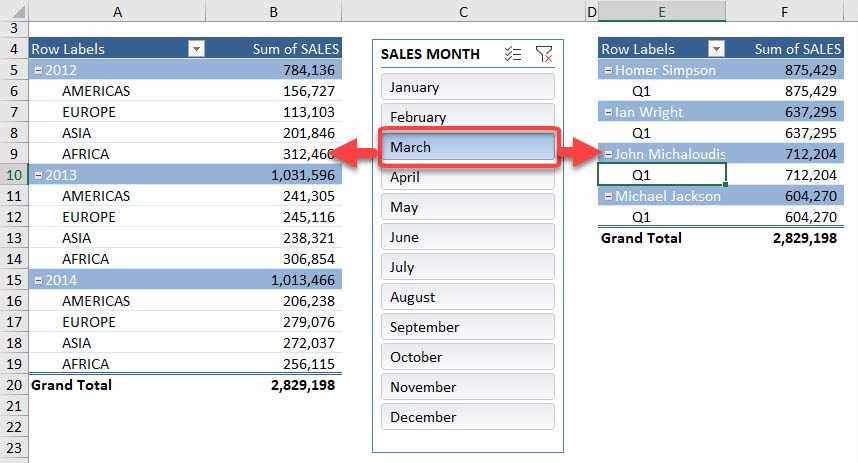
STEP 2: Click in Pivot Table #1 and insert a MONTH Slicer by going to PivotTable Tools > Analyze/Options > Insert Slicer > Month > OK


STEP 3: Click in Pivot Table #2 and insert a YEAR Slicer by going to PivotTable Tools > Analyze/Options > Insert Slicer > Year > OK


STEP 4: Right Click on Slicer #1 and go to Report Connections(Excel 2013, 2016, 2019 & Office 365)/PivotTable Connections (Excel 2010) > “check” the PivotTable2 box and press OK


STEP 5: Right Click on Slicer #2 and go to Report Connections(Excel 2013, 2016, 2019 & Office 365)/PivotTable Connections (Excel 2010) > “check” the PivotTable1 box and press OK


Now as you select each Slicer’s items, both Pivot Tables will change!

Troubleshooting Common Slicer Connection Issues
Things to Check in Slicer-Pivot Table Integration
Maybe the slicer isn’t influencing all your intended tables, or perhaps it’s acting up entirely. To smooth things over, start by double-checking that all pivot tables originate from the same data source or are connected through the Power Pivot Data Model.
You can check your slicer by right-clicking and selecting ‘Report Connections’. Based on the list, make sure every table you want controlled by the slicer is checked off.
Frequently Asked Questions
What is a slicer in excel?
A slicer in Excel is a visual tool that lets you filter pivot tables, charts, or tables with the simple click of a button. It’s perfect for when you need to break down a hefty dataset into more digestible pieces, without the need to navigate complex menus.
How Do I Connect a Slicer to Several Pivot Tables?
Connecting a slicer to several pivot tables can be done in a few straightforward steps. After inserting a slicer connected to one pivot table, you can easily extend its influence to others. Right-click on the slicer and select ‘Report Connections’ or ‘Pivot Table Connections’, depending on your Excel version. In the dialog box that pops up, you’ll see a list of all pivot tables in your workbook. Here, simply check the boxes next to the pivot tables you wish each slicer to control, and press ‘OK’. Voila! Your slicer will now apply its filter across all selected pivot tables, enabling a synchronized data experience.
Can I Customize Slicer Options for Different Pivot Tables?
Absolutely! Each slicer comes with a suite of customizable options to tailor the look and feel for different pivot tables. This means you can adjust colors, button styles, and even how many columns of buttons appear in the slicer for improved readability and match your workbook’s aesthetic.
Fine-tune your slicer’s settings by selecting it and navigating to the Slicer Tools Options tab on the Excel ribbon. Here you can craft unique styles or pick from Excel’s gallery of built-in designs. And for those extra-special touches, remember, you can customize things further such as the visually distinctive “tabs” effect, by tinkering with border and fill colors that echo your pivot table headers.

John Michaloudis is a former accountant and finance analyst at General Electric, a Microsoft MVP since 2020, an Amazon #1 bestselling author of 4 Microsoft Excel books and teacher of Microsoft Excel & Office over at his flagship MyExcelOnline Academy Online Course.


