Consolidate Multiple Excel Workbooks Using Power Query

One of the most sought after a query from the millions of Excel users around the world is:  How do I consolidate multiple Excel workbooks in Power Query into one?  There are a couple of ways you can do this, using VBA or complex formulas but the learning curve is steep and out of reach for most Excel users. Luckily with Power Query Excel Workbook, this consolidation task can be done in a couple of minutes!  That’s right, only a couple of minutes.

Key Takeaways

• Import Multiple Files Easily – Power Query can load all Excel files from a folder in one go, saving time on manual copying.

• Automate Consolidation Tasks – Once set up, the query can refresh automatically when new files are added to the folder.

• Standardized Structure Required – All workbooks must have a consistent layout (same sheet/table structure) to consolidate properly.

• Transform and Clean Data Before Combining – Power Query allows filtering, removing columns, renaming headers, and more before merging.

• Output Combined Data to One Table – The final result can be loaded into an Excel sheet or Data Model for reporting and analysis.

How to Consolidate Multiple Excel Workbooks Using Power Query

STEP 1: Create a New Folder on your Desktop or any directory and name it to whatever you like e.g. 2016 Sales

Move an Excel Workbook in this Folder that contains your Sales data e.g. January 2016.xlsx

 

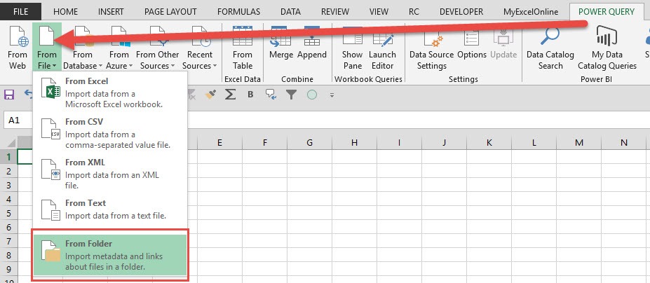
STEP 2: Open a NEW Excel Workbook and go to Power Query > From File > From Folder

 

STEP 3: From the Folder dialogue box, click the Browse button

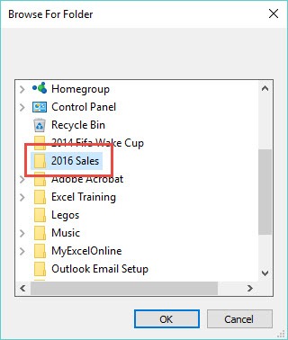
This will bring up the Browse for Folder dialogue box and you need to select the folder you created in Step 1 and press OK.

This is how you can use Power Query load multiple files from folder feature.

 

STEP 4: This will open up the Query Editor.

From in here you need to select the first 2 columns (hold down the CTRL key to select) and Right Click on the column heading and choose Remove Other Columns

 

STEP 5: You need to go to Add Column > Add Custom Column

 

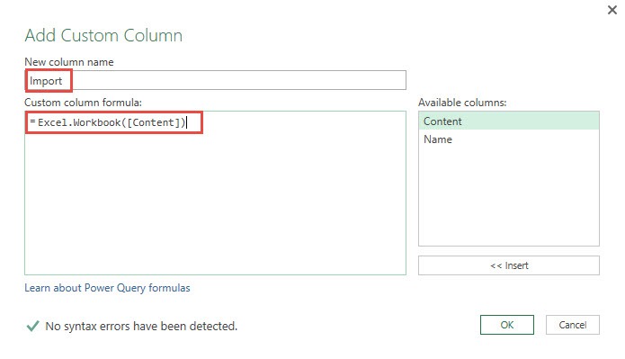
STEP 6: This will bring up the Add Custom Column dialogue box.

In here you need to name the new column E.G. Import, and within the Custom Column Formula you need to enter the following formula:

= Excel.Workbook([Content])

This will import the workbooks from within the Folder that you selected in Step 3

 

STEP 7: You now have a new column called Import.

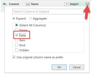
Click on the Expand Filter and select the Data box only and press OK.  This will import the workbook from the folder

 

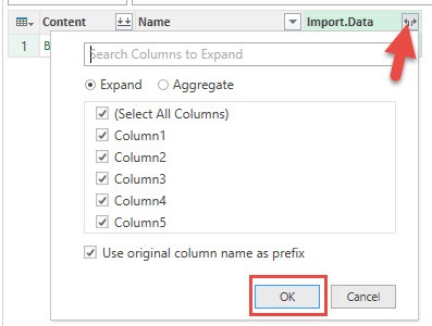
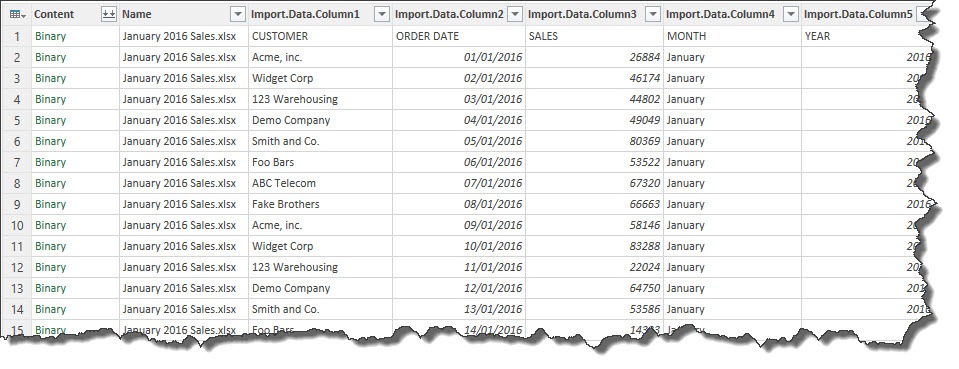
STEP 8: Click on the Expand Filter from the Import Data column and select OK.  This imports all the columns’ data from within the workbook

 

STEP 9: Now it is time to transform the data by making some cosmetic changes!

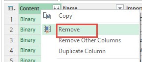
Remove the Content column by Right-Clicking and choosing Remove

 

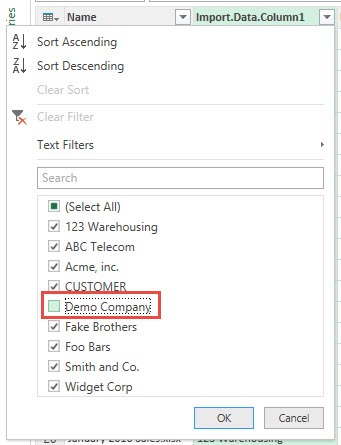
STEP 10: Select the Import.Data.Column1 and filter out the CUSTOMER heading and press OK.  This will also remove the other column’s headers

 

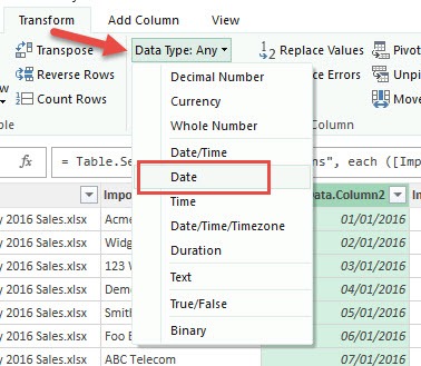
STEP 11: Select the Date column and go to Transform > Data Type > Date

 

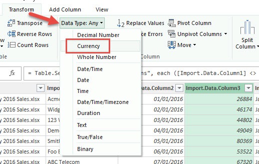
STEP 12: Select the Sales column and go to Transform > Data Type > Currency

 

STEP 13: Rename the column headings to whatever you like by double clicking on the column header, renaming and pressing OK

 

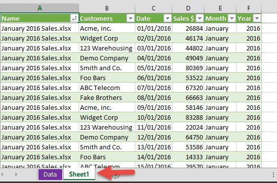
STEP 14: Go to File > Close & Load.

 

This will put the data into a new worksheet within your workbook

 

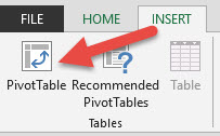
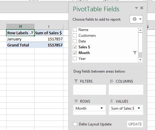
STEP 15: You can now Insert a Pivot Table to do your analysis by going to Insert > Pivot Table > New/Existing Worksheet

 

Put the Months in the ROWS and the Sales $ in the VALUES area:

 

STEP 16: NOW FOR THE COOL PART!!!!

You can move similar workbooks into the Folder we created in Step 1, say for subsequent months eg. February 2016.xlsx, March 2016.xlsx etc

NB: The Excel Workbooks have to have the same format and number of columns as in the workbook we imported in Step 1

 

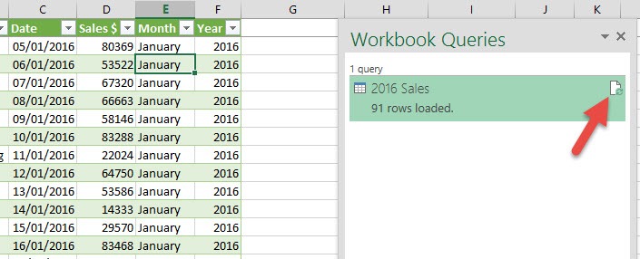
STEP 17: In your Excel workbook, click on the imported data and this will open up the Workbook Queries pane (If this does not open, go to Power Query > Show Pane)

Click the Refresh button (or you can go to Table Tools > Query > Refresh)

 

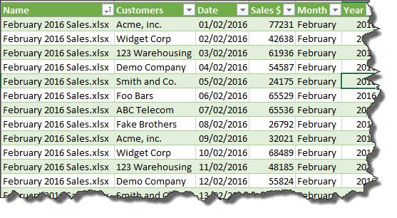
STEP 18: This will import the February 2016.xlsx and March 2016.xlsx data into the Excel workbook and append it to January’s data

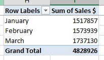
STEP 19: Now you can Refresh the Pivot Table and the new imported data will be reflected

 

Next month all you have to do is drop in the new month’s workbook into the 2016 Sales Folder and Refresh the Query & the Pivot Table to see the results!

THAT IS POWER!!!!

Frequently Asked Questions

Do all the Excel workbooks need to have the same format?
Yes, they should have identical column headers and data structure for the consolidation to work correctly.

Can I consolidate files stored in different folders?
Power Query works best when files are in a single folder, but you can repeat queries for each folder and then merge them.

Will changes in the source files be reflected automatically?
Yes, after clicking Refresh All in Excel, Power Query will reload and update the consolidated data.

Can I exclude certain files or sheets from the folder?
Yes, during the query setup, you can apply filters based on file name, date modified, or sheet name.

Is Power Query available in all versions of Excel?
Power Query is built-in from Excel 2016 onward. For Excel 2010 and 2013, it can be added as a free add-in.