Sum a Range Using the INDEX Function

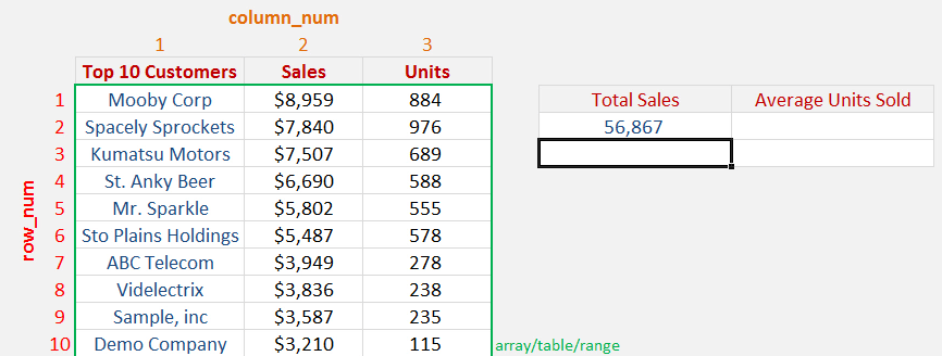
You can sum a range of values within a table using the INDEX function in Excel.  This is valuable when you want to extract key metrics from a table and put them in an Excel Dashboard. To make this work you first need to start your Excel formula with the SUM Index Match.

So it will look something like this:  =SUM(INDEX(Array, Row_Num, Column_Num))

The Array will be your table of data, the Row_Num will be blank, and the Column_Num will be the column number where you want to SUM the values.

When we dissect the formula (by highlighting the INDEX function and pressing F9) we can see that the following is happening: =SUM({8959;7840;7507;6690;5802;5487;3949;3836;3587;3210})

So, in effect, we are summing the array of values within the table.  See the example below that shows you how this is done.

Key Takeaways

• Create Flexible Ranges – INDEX allows you to define dynamic start and end points within a range for summing.

• Avoid Hardcoding Ranges – Using INDEX helps build formulas that adapt as your data grows or changes.

• Combine with SUM Function – Nest INDEX inside SUM to calculate totals over changing segments of a dataset.

• Useful for Dynamic Dashboards – Great for summing values between two lookup positions without helper columns.

• Works with Named Ranges Too – INDEX can be used on both normal and named ranges for cleaner formulas.

 

Introduction to the INDEX Function

The INDEX function returns the value of a cell in a table based on its row and column numbers. Unlike other lookup functions, such as VLOOKUP or HLOOKUP, the INDEX function gives me much more flexibility when dealing with data spread across both rows and columns.

The syntax for the INDEX function is:

=INDEX(array, row_num, [column_num])

• array: This is the range of cells or array from which I want to retrieve data.
• row_num: This is the row number in the array.
• column_num: (Optional) This is the column number in the array.

 

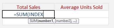
STEP 1: We need to place first the INDEX function inside the SUM function.

=SUM(INDEX

 

The Index arguments:

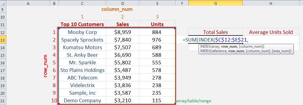
array

What is the range/table?

Reference the range of cells here that we want to get the values from:

=SUM(INDEX($C$12:$E$21,

 

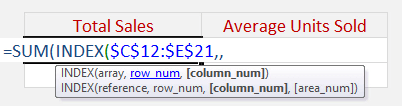
row_num

What is the row number we want to return?

We do not need to return the row, as we want to just sum all of the sales. Leave the row number blank:

=SUM(INDEX($C$12:$E$21,,

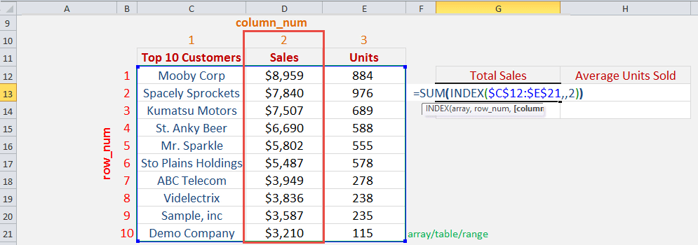
column_num

What is the column number we want to return?

Since we want the sales column, this is column number 2. So place in 2:

=SUM(INDEX($C$12:$E$21,,2))

Instead of providing column_num, you can also use the sum with index match function!

 

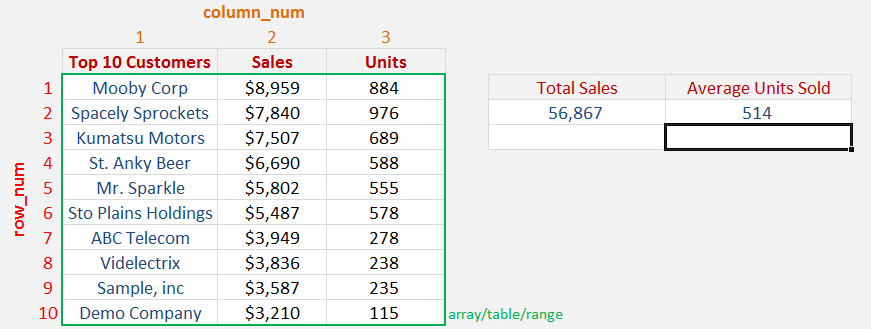
Now you are able to get the Total Sales:

 

STEP 2: Now let us try how we can use this with the AVERAGE function. We need to place first the INDEX function inside the AVERAGE function.

=AVERAGE(INDEX

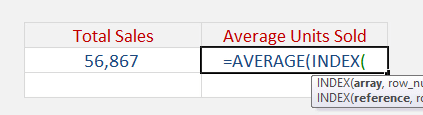
The Index Function Excel arguments:

array

What is the range/table?

Reference the range of cells here that we want to get the values from:

=AVERAGE(INDEX($C$12:$E$21,

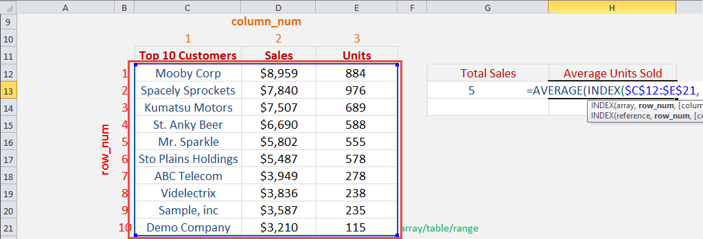
row_num

What is the row number we want to return?

We do not need to return the row, as we want to just average all of the units. Leave the row number blank:

=AVERAGE(INDEX($C$12:$E$21,,

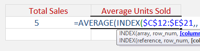
column_num

What is the column number we want to return?

Since we want the units column, this is column number 3. So place in 3:

=AVERAGE(INDEX($C$12:$E$21,,3))

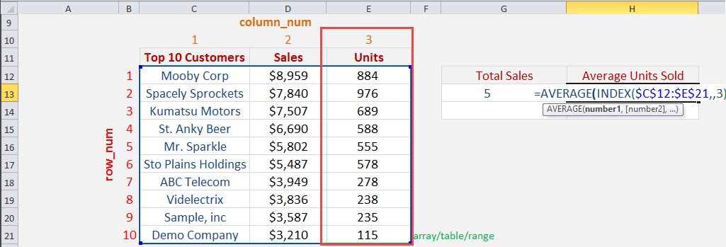
Instead of providing column_num, you can also use the index match sum or index match sum multiple rows!

 

Now you are able to get the Average Units Sold:

 

Using the OFFSET Function to Sum a Dynamic Range

You can also use the OFFSET function to create a dynamic range in Excel. You can combine OFFSET with the SUM function to add values from a changing range.

The syntax for the OFFSET function is:

=OFFSET(reference, rows, cols, [height], [width])

For example, you can use the following formula:

=SUM(OFFSET(C12,0,1,10,1))

Here is how the formula works:

• C12 is the starting cell.
• 0 means you do not move any rows from C12.
• 1 moves one column to the right to the Sales column.
• 10 includes 10 rows in the range.
• 1 includes one column.

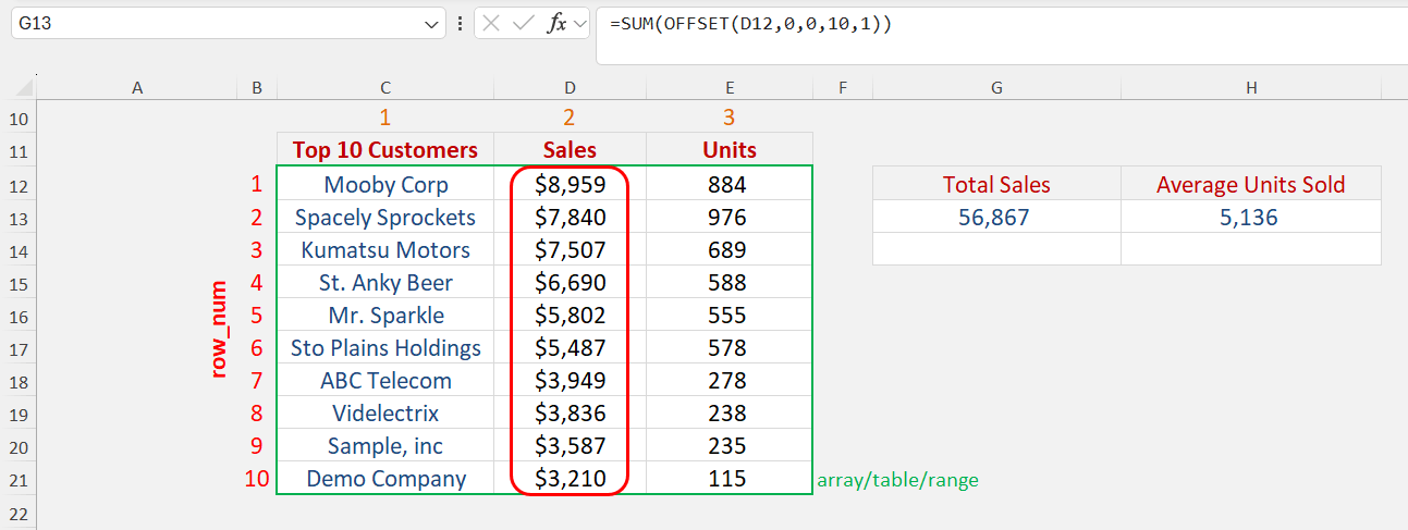
The OFFSET function returns 10 cells from the Sales column. The SUM function then adds all the values in the returned range.

 

FAQs