In Power Pivot, one of the major and more powerful feature are Measures.
Measures (also known as Calculated Fields in Excel 2013) are formulas/calculations that are added to a Pivot Table.
We will work on a simple example to show you how easy it is to add your first Measure.
Table of Contents
Want to learn about Measures vs Calculated Columns in Power Pivot?
*** Watch our video and step by step guide below with free downloadable Excel workbook to practice ***
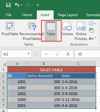
STEP 1: Select the Sales Table. Go to Insert > Table. Click OK.
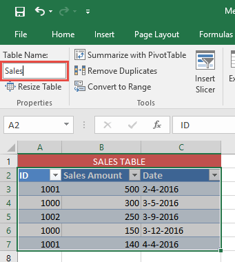
STEP 2: Go to Table Tools > Design > Table Name and give your new Table a descriptive name. In our example, we will name it Sales
STEP 3:
In Excel 2013 & 2016
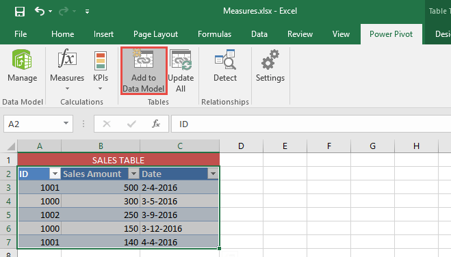
Select your Sales Table. Go to Power Pivot > Add to Data Model.
This will import your new Table into the Power Pivot Window.
In Excel 2010
Go to PowerPivot > Create Linked Table.
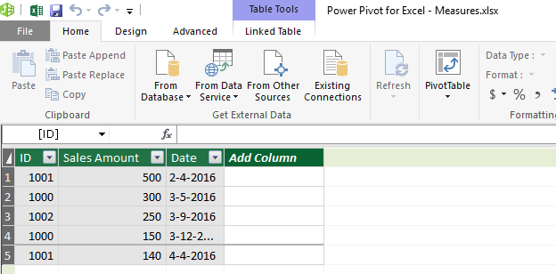
STEP 4: This will open the Power Pivot Window.
The Sales Table will now be automatically loaded to the Power Pivot Data Model.
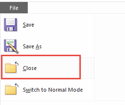
Now Close the Power Pivot Window.
STEP 5: Go to Insert> Pivot Table.
In Excel 2016
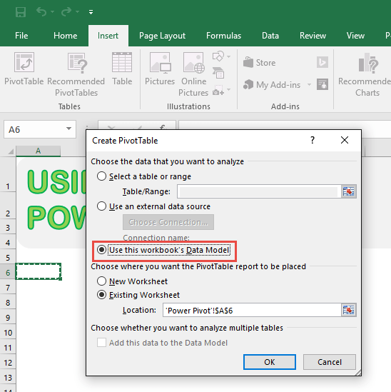
Select Use this workbook’s Data Model. This will use the Data Model you just uploaded in the last step.
Select Existing Worksheet and choose your location for your Pivot Table and press OK.
In Excel 2013
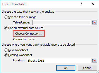
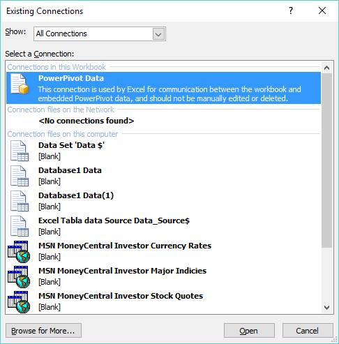
Go to Use External Data Source > Choose a Connection
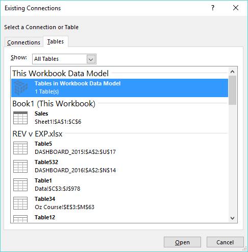
Now select Tables > This Workbooks Data Model > Open:
In Excel 2010
Go to Use an External Data Source > Choose Connection:
Now select PowerPivot Data > Open:
STEP 6: Adding a Measure:
In Excel 2016
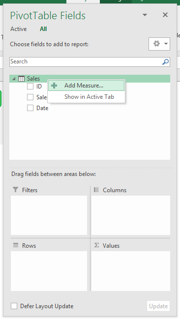
On the Sales Table, right click and select Add Measure.
An alternative way in Excel 2016 is go to Power Pivot > Measures > New Measure.
In Excel 2013
Go to PowerPivot > Calculated Fields > New Calculated Field
(In Excel 2013 “Measures” were renamed “Calculated Fields” and returned to “Measures” in Excel 2016…I know, how annoying!)
In Excel 2010
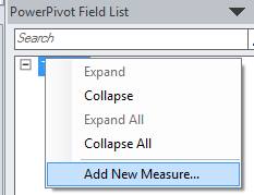
On the Sales table, right click and select Add New Measure.
An alternative way in Excel 2010 is to select a cell inside the Pivot Table that was created in the previous step and go to Power Pivot > New Measure:
STEP 7: This is where we create our first Measure.
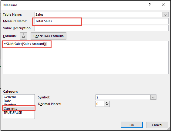
For Measure Name, type in any name that you like e.g. Total Sales
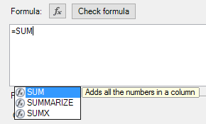
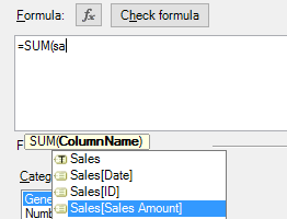
For the Formula, after the = sign start typing the word SUM.
Just like in native Excel, this will bring up the Formula helper and choose the SUM function by either double clicking on the blue highlighted SUM option or by pressing the Tab keyboard to confirm this suggestion:
After the SUM formula is selected, type in the Table name that we created in Step 2, which we called Sales.
This will bring up the Formula helper and within here you need to select the Sales [Sales Amount] option and close the parenthesis:
Set the Category as Currency, and this will automatically handle the formatting for you. Press OK to confirm this.
This Measure will now return the Sum Total of the Sales Amount column within the Sales Table.
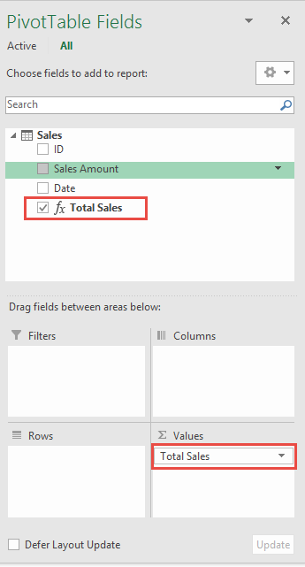
STEP 8: Place your new Measure Total Sales in the Values area.
STEP 9: Now we are able to use our new Measure in the Pivot Table.
Further Learning:

Bryan
Bryan is a best-selling book author of the 101 Excel Series paperback books.


