Create Custom Symbols in Excel based on Numbers

In this tutorial, you will be provided with detailed guidance to:

• Understanding the Number Format Code

• Create Custom Symbols in Excel

Watch it on YouTube and give it a thumbs-up!

Excel has several in-built features to create custom formatting to your numbers. But if none of them meets your requirement, you will have to create your own.

The key benefit of adding custom formatting is that it only controls how the number is displayed without changing the underlying value of that number.

A cool feature within Excel is the ability to format a cell’s value by pressing CTRL + 1 on any cell. This brings up the Format Cells dialogue box and under the Custom category, you can customize the Type to whatever you like.

You can even create custom symbols in Excel using this feature!

But before you understand how to add a symbol to a number in Excel, you need to first know how to write a number format code.

Understanding the Number Format Code

You can change the format of a cell’s value by either using various formats available in Excel or creating a custom format using number format code.

Number format code is created using symbols that tells Excel how you want to display the cell’s value. When adding a custom format in Excel, there are four formatting sections that you have to follow:

Positive format; Negative format; Zero format; Text format. 

Each of these sections is separated by a semicolon(;) and only the first section is required to create a custom format.

You can view the Custom Number Formats blog post that explains this in more detail here

Create Custom Symbols in Excel

Now that you have understood the structure of how to use number format code, let’s use that knowledge and learn how to insert symbol in excel formula based on the cell’s value.

Working with an example will make this concept more clear. So, let’s get started.

Follow the step-by-step tutorial below to know how to add a symbol in excel formula and make sure to download the exercise workbook to follow along:

DOWNLOAD EXCEL WORKBOOK

Example #1:

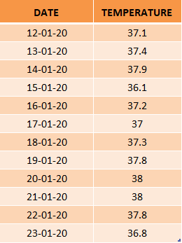
In the table below, you have daily temperature recorded and you want to add symbol °C to it.

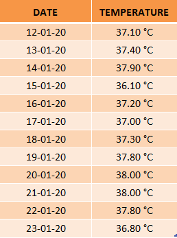
You want to add “°C” symbol to the temperature column and the edited table like this:

The following steps should be incorporated to create custom symbols in Excel:

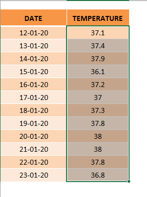
STEP 1: Select the “Temperature” column

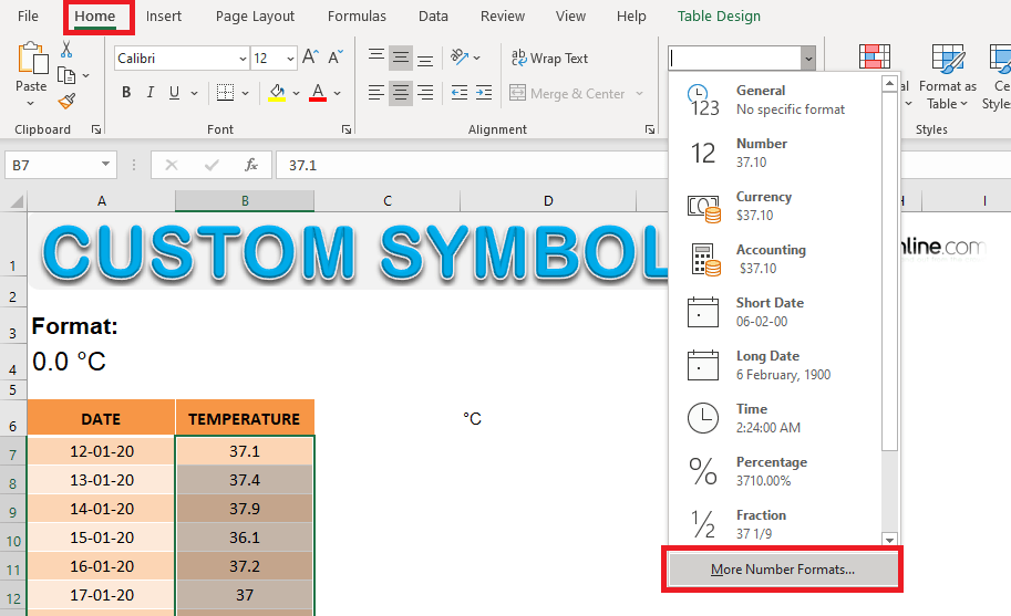
STEP 2: Go to Home > Under Format Dropdown, Select More Number Formats

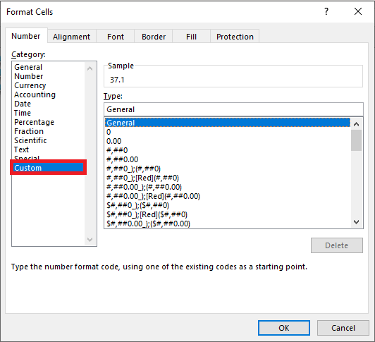
STEP 3: In the Format Cell dialog box, select Custom

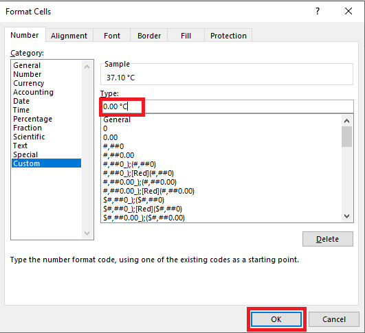
STEP 4: In the type section, type 0.00 °C and Click OK

This is how the edited table will look like.

Example #2: 

In Example #1, you have learned how to add symbols in Excel irrespective of the cell’s value. Now let’s move forward and understand how to add symbols based on the number stored in the cell.

So, the symbols added would be based on the value stored in the cell.

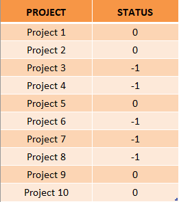
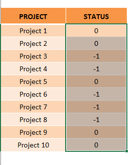
In the table below, you have the status for different projects listed below with “0″ indicating Completed and “-1” indicating Pending.

Now you want to create custom symbols in Excel i.e. you want to add custom symbol :

• ✓ Completed; when status is 0
• ✕ Pending; when status is -1

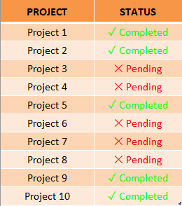
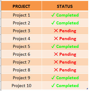
The table with custom symbols should look like this:

STEP 1: Select the Status Column

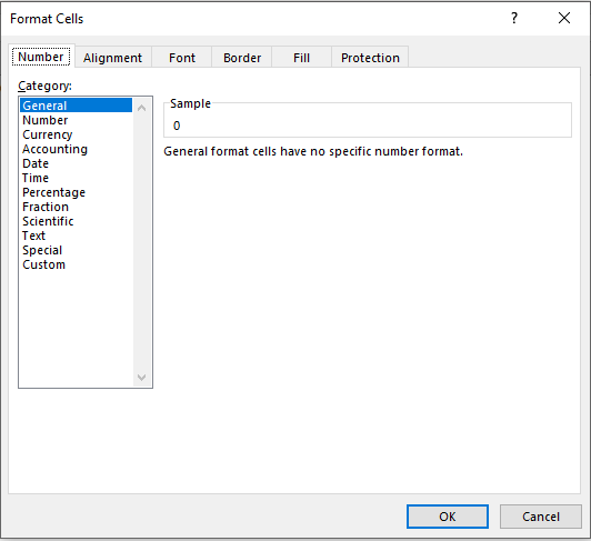
STEP 2: Press Ctrl +1 to open the Format Cells dialog box

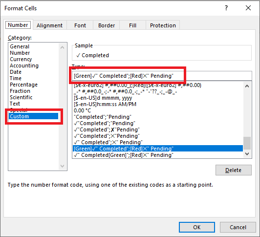
STEP 3: Select the Custom category and select a number format type – ✓” Completed”;✕” Pending”. This will change the format to ✓ Completed when cell value is 0 and ✕ Pending when cell value is -1.

You can also add color to make the formatting more distinct. Use the format type –  ✓” Completed”[Green];[Red]✕” Pending” to add green color to the completed project and red to pending projects.

This is how the table will look like this.

Example #3: 

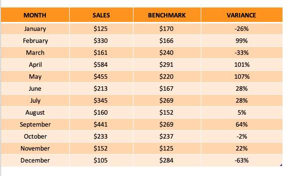
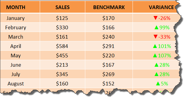
Here, you have monthly sales, estimates benchmark sales and variance calculated.

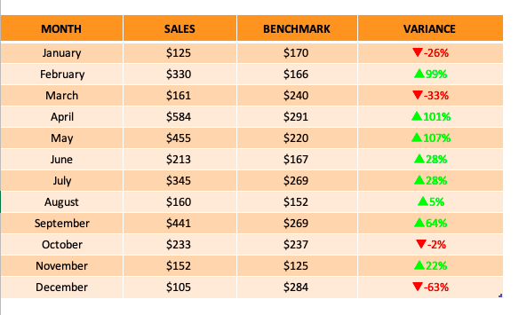
You want the % Variance column in our data to have symbols ▲▼ to show a negative and positive variance. So, you have the % variance value customized as below:

• Green in color with ▲ symbol; when variance % is positive
• Red in color with ▼ symbol; when variance % is negative

The table should look something like this:

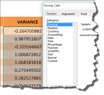
STEP 1: Enter a Variance calculation in a column, select the column’s variance numbers and press CTRL + 1 to bring up the Format Cells dialogue box

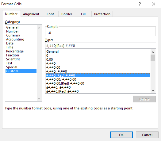
STEP 2: Select the Custom category and select a number format type – “#,##0;[Red]-#,##0

The first section of this code #,##0 is for a positive number, and second code [Red]-#,##0 is for a negative number.

To show the positive number in green color and add a % sign, follow Step 3.

STEP 3: Under the Type: area you will need to enter the text [green] at the start of the positive value string and enter the % sign at the end of the positive and negative value strings

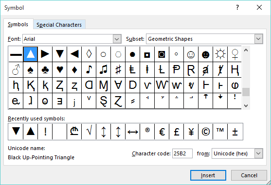
STEP 4: Now select a blank cell and go to Insert > Symbol > Font: Arial > Subset: Geometric Shapes and then Insert the Up-Pointing Triangle and Insert the Down-Pointing Triangle and press Cancel

STEP 5: You will need to copy the triangles, select the variance numbers, press CTRL + 1 and paste the triangles before each positive and negative value string, then press OK

You now have your custom number formats with an upwards triangle for any positive %s and a downwards triangle for any negative %s

Further Learning:

• Add a Degree Symbol to Selection Using Macros In Excel
• Top 3 Methods to Find Special Characters in Excel
• Turn Text To Values With Paste Special Values

Make sure to download our FREE PDF on the 333 Excel keyboard Shortcuts here:

You can learn more about how to use Excel by viewing our FREE Excel webinar training on Formulas, Pivot Tables, and Macros & VBA!

You can follow our YouTube channel to learn more about How To Use Excel efficiently!