But we can use different functions or a combination of functions to extract any particular string. A few substring functions that we can use in Excel are:
Let’s look into each of these functions one by one. You can also download the Excel Workbook and follow along.
The LEFT function can be used to extract a specified number of characters from the left of the text string.
LEFT(text, [num_chars])
- text – It refers to the text string that contains the characters you want to extract.
- num_chars – Optional. Specifies the number of characters you want LEFT to extract.
- Num_chars must be greater than or equal to zero.
- If num_chars is greater than the length of the text, LEFT returns all of the text.
- If num_chars is omitted, it is assumed to be 1.
In this example, we want to extract the first 3 characters from our reference text string in cell A2.
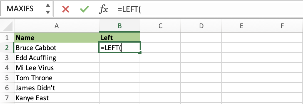
STEP 1: We need to enter the Left function next to the cell that we want to extract the data from:
=LEFT(
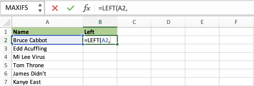
STEP 2: Enter the first argument – text. This is the reference cell that contains the text or value from which you want to extract X characters.
=LEFT(A2
STEP 3: Enter the second argument – [num_chars]. This is the number of characters you want to extract from cell A2. Enter a positive number only.
=LEFT(A2, 3)
The RIGHT function can be used to extract a specified number of characters from the right of the text string.
RIGHT(text,[num_chars])
- text – It refers to the text string that contains the characters you want to extract.
- num_chars – Optional. Specifies the number of characters you want RIGHT to extract.
- Num_chars must be greater than or equal to zero.
- If num_chars is greater than the length of the text, RIGHT returns all of the text.
- If num_chars is omitted, it is assumed to be 1.
In this example, we want to extract the last 4 characters from our reference text string in cell A2.
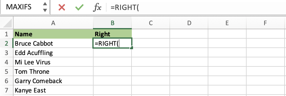
STEP 1: We need to enter the RIGHT function next to the cell that we want to extract the data from:
=RIGHT(
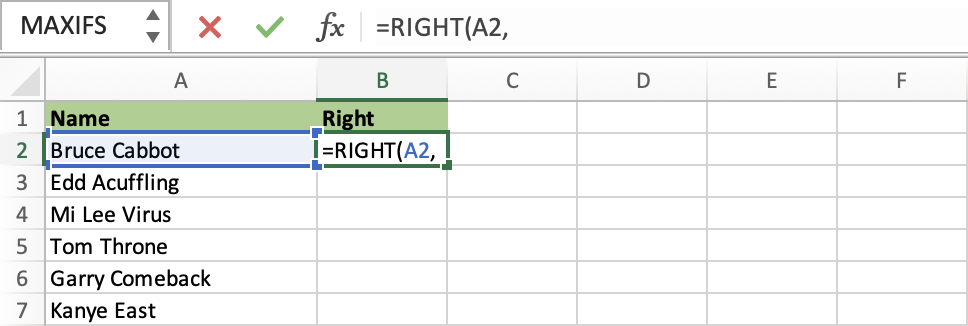
STEP 2: Enter the first argument – text. This is the reference cell that contains the text or value from which you want to extract X characters.
=RIGHT(A2,
STEP 3: Enter the second argument – [num_chars]. This is the number of characters you want to extract from cell A2. Enter a positive number only.
=RIGHT(A2, 4)
The MID function can be used to extract a specified number of characters from the specified starting position in a text string.
MID(text,start_num,num_chars)
- text – It refers to the text string that contains the characters you want to extract.
- start_num – It is the position of the first character you want to extract from the text. The first character in the text has start_num 1, and so on.
- num_chars – specifies the number of characters you want MID to return from the text.
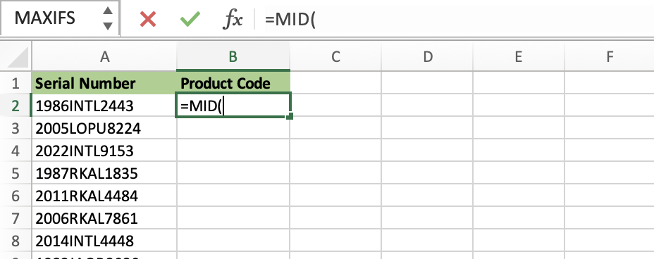
In this example, we want to extract 4 characters starting from the 5th position of the text string.
STEP 1: Enter the MID function in a blank cell.
=MID(
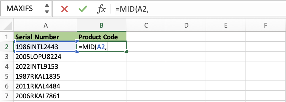
STEP 2: Enter the first argument – text. Select the cell containing the source text that you want to extract from –
=MID(A2,
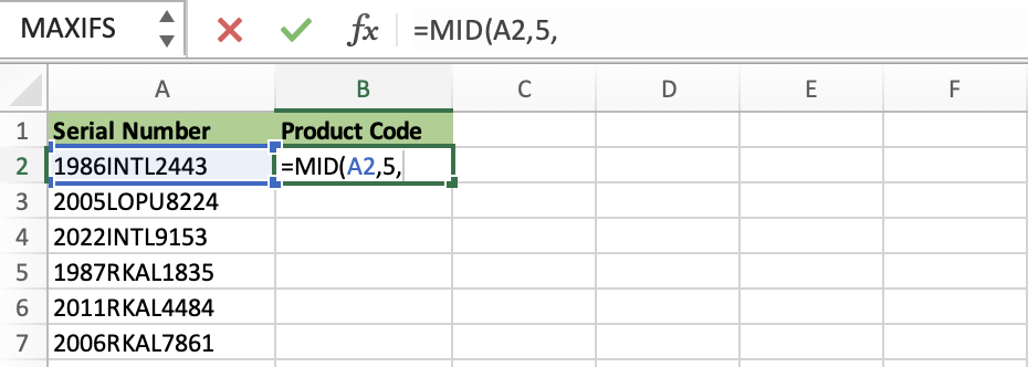
STEP 3: Enter the second argument – start_num
Enter the starting position – This is where the MID formula will start getting the text.
=MID(A2, 5,
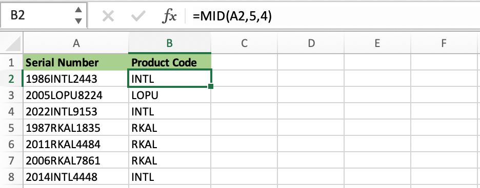
STEP 4: Enter the third argument – num_chars
Enter the number of characters you want to extract. In our case, we want to get 4 characters.
=MID(A2, 5, 4)
The LEN function can be used to return the number of characters in the text string.
LEN(text)
- text – It refers to the text string from which you want to get the number of characters
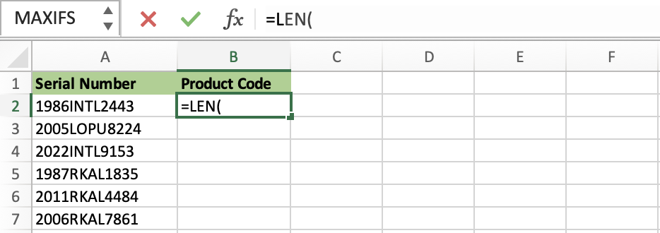
In this example, we want to extract the number of characters in the text string.
STEP 1: Enter the LEN function next to the cell that we want to get the number of characters from
=LEN(
STEP 2: Enter the first argument – text
=LEN(A2)
The FIND function can be used to get the position of a specific text within another text.
FIND(find_text, within_text, [start_num])
- find_text – It is the text that needs to be searched
- within_text – It is the source text
- start_num – It is the starting position of the source text
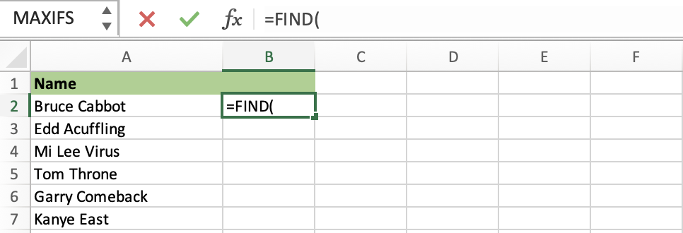
In this example, we want to find the position or location of space (“ “) in the text string mentioned in cell A2.
STEP 1: We need to enter the FIND function in a blank cell:
=FIND(
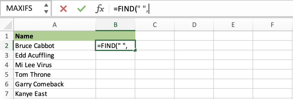
STEP 2: Enter the first argument – find_text. Enter the character that you need to search for in the source text. In our case, it is a space (” “).
=FIND(” “,
STEP 3: Enter the second argument – within_text. Select the cell containing the source text.
=FIND(” “, A2)
STEP 4: Enter the third argument – [start_num]
This is the position from which you want to start searching in your source text. You can leave this blank, it will default to 1 which means it will start looking from the first character of your source text.
The TRIM function can be used to remove unneeded spaces in your text, except single spaces in between words.
TRIM(text)
- text – It is the text from which you want extra spaces to be removed
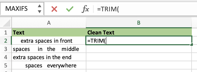
Extra spaces are very difficult to spot, especially those at the end. In this example, all the extra spaces from the text whether it be from the start, middle, or at the end of the text have been removed.
All the unneeded spaces in the text, except single spaces between words have been removed.
STEP 1: We need to enter the Trim function
=TRIM(
STEP 2: Enter the argument – text. This is the source text from which you want to remove extra spaces.
=TRIM(A2)
TEXTBEFORE function can be used to extract the text that occurs before a given character or string. It is available in Excel 365 only.
TEXTBEFORE(text,delimiter,[instance_num], [match_mode], [match_end], [if_not_found])
- text – It is the text you are searching within.
- Wildcard characters are not allowed.
- If the text is an empty string, Excel returns empty text.
- delimiter – It is the text that marks the point before which you want to extract.
- instance_num – It is the instance of the delimiter after which you want to extract the text.
- By default, instance_num = 1.
- A negative number starts searching for the text from the end.
- Optional.
- match_mode – It determines whether the text search is case-sensitive. The default is case-sensitive. Optional. Enter one of the following:
- 0 Case sensitive.
- 1 Case insensitive.
- match_end – It treats the end of the text as a delimiter. By default, the text is an exact match. Optional. Enter the following
- 0 – Don’t match the delimiter against the end of the text.
- 1- Match the delimiter against the end of the text.
- if_not_found – It is the value returned if no match is found. By default, #N/A is returned. Optional.
In the example, we have provided the cell containing the text string and the delimiter (i.e. space) as arguments and the function provides us with first names as result.
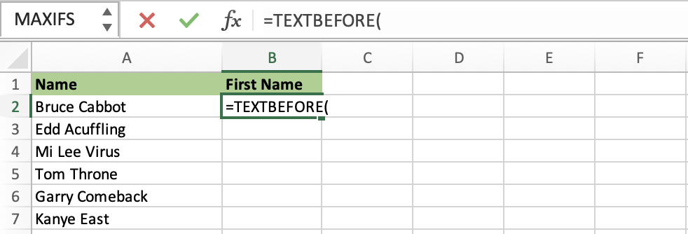
STEP 1: Enter the TEXTBEFORE function
=TEXTBEFORE(
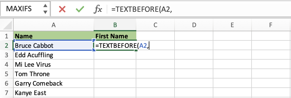
STEP 2: Enter the first argument – text. Enter the source text from which you want to extract a substring.
=TEXTBEFORE(A2,
STEP 3: Enter the second argument – delimiter. This is the character that marks the point before which you want to extract. In our case, the delimiter is a space.
=TEXTBEFORE(A2,” “)
All the first names have been easily extracted in column B.
If you do not have this function in Excel, you can also try a combination of the LEFT and FIND functions to get the first names. Let’s give it a try.
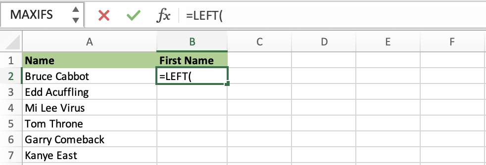
STEP 1: Enter the LEFT function
=LEFT(
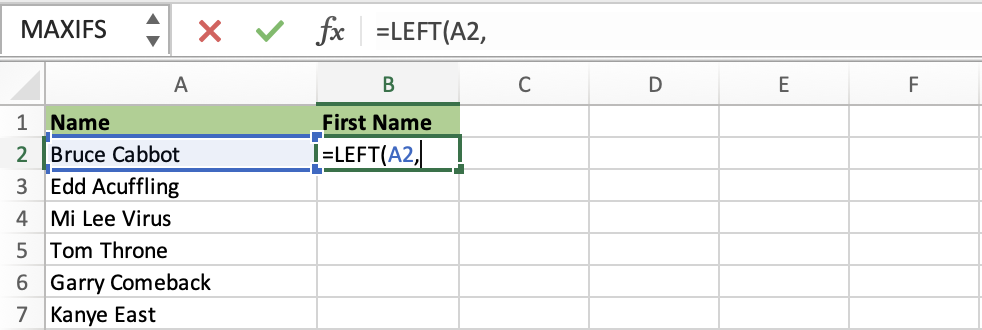
STEP 2: Enter the first argument of the LEFT function – text. This is the source text from which you want to extract a substring.
=LEFT(A2,
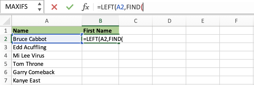
STEP 3: Enter the FIND function. This function is used to find the position of space in our source text.
=LEFT(A2,FIND(
STEP 4: Enter the first argument of the FIND function – find_text. This is the character that you need to search for in the source text. Here, it is a space (” “).
=LEFT(A2,FIND(” “,
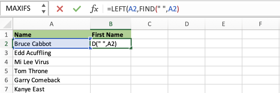
STEP 5: Enter the second argument of the FIND function – within_text. This is the cell containing the source text.
=LEFT(A2,FIND(” “,A2)
STEP 6: Subtract 1.
We are subtracting 1 from the delimiter’s position to get the number of characters before the delimiter. This will give us the number of characters for the first name.
=LEFT(A2,FIND(” “,A2)-1)
We have used the left and find functions to simply extract those characters from the left of space i.e. the first name.
The TEXTBEFORE function has a complementary function for substring needs in EXCEL, i.e., TEXTAFTER. This function returns text that occurs after a given character or string.
TEXTAFTER(text,delimiter,[instance_num], [match_mode], [match_end], [if_not_found])
In the example, we have provided the cell reference containing the text string and the delimiter (i.e. space) as arguments and the function provides us with the result. All the last names have been easily extracted in column B.
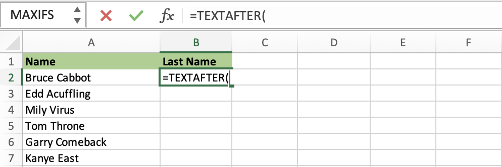
STEP 1: Enter the TEXTAFTER function
=TEXTAFTER(
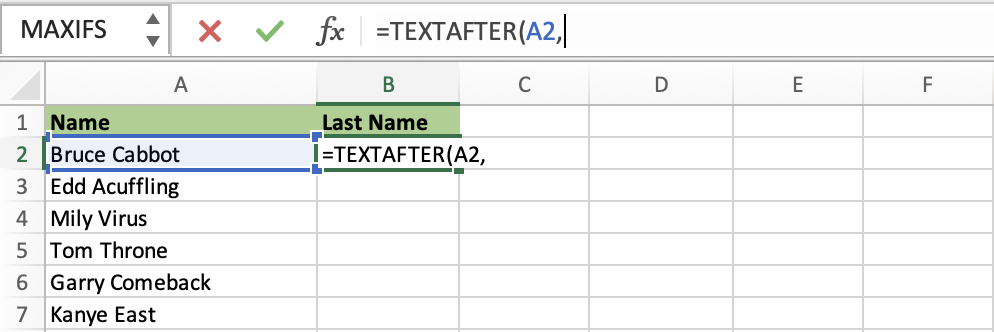
STEP 2: Enter the first argument – text. Enter the source text from which you want to extract a substring.
=TEXTAFTER(A2,
STEP 3: Enter the second argument – delimiter. This is the character that marks the point after which you want to extract. In our case, the delimiter is a space.
=TEXTAFTER(A2,” “)
If you do not have this function in Excel, you can also try a combination of RIGHT, LEN, and FIND functions to get the last names. Let’s give it a try.
First, we need to count the number of characters in the entire text string using the LEN function. Then, we can subtract the positional number at which our delimiter is. This will give us the number of characters left after the delimiter.
Then, the right function simply extracts those numbers of characters from the reference text string.
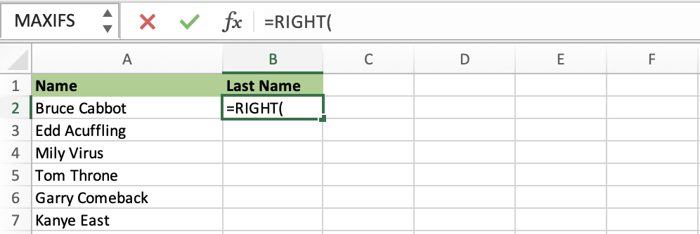
STEP 1: Enter the RIGHT function
=RIGHT(
STEP 2: Enter the first argument of the RIGHT function – text. This is the source text from which you want to extract a substring.
=RIGHT(A2,
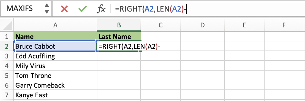
STEP 3: Enter the LEN function. This function is used to find the total number of characters in our source text.
=RIGHT(A2,LEN(A2)
STEP 4: Enter the subtract symbol
=RIGHT(A2,LEN(A2)-
STEP 5: Enter the FIND function.
=RIGHT(A2,LEN(A2)-FIND(
STEP 6: Enter the first argument of the FIND function – find_text. This is the character that you need to search for in the source text. Here, it is a space (” “).
=RIGHT(A2,LEN(A2)-FIND(” “,
STEP 7: Enter the second argument of the FIND function – within_text. This is the cell containing the source text.
=RIGHT(A2,LEN(A2)-FIND(” “,A2))
John Michaloudis is a former accountant and finance analyst at General Electric, a Microsoft MVP since 2020, an Amazon #1 bestselling author of 4 Microsoft Excel books and teacher of Microsoft Excel & Office over at his flagship MyExcelOnline Academy Online Course.

