How to Deduct 90 Days Before Today in Excel

In Excel, calculating dates is a common task that can be accomplished with various functions and formulas. Calculating 90 days before today can be particularly useful for project management, financial analysis, or tracking deadlines. Here’s a step-by-step guide on how to achieve this using Excel.

Key Takeaways:

• Use the TODAY() function in Excel to get the current date instantly and keep your data updated.
• Subtract 90 days from today’s date with the formula =TODAY()-90 for quick and accurate historical insights.
• Use the EDATE() function for more complex date calculations involving months.
• Format cells to display dates correctly by selecting the “Date” category in the “Format Cells” menu.
• Highlight important dates using conditional formatting with formulas like =B2>TODAY()-90 to create visual cues for time-sensitive tasks.

 

Discovering Time with Excel’s Date Functions

The Magic of TODAY() and EDATE()

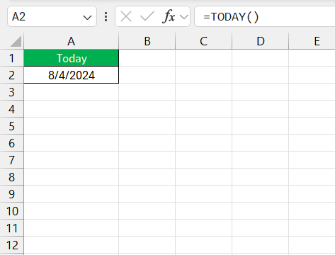
In the realm of Excel, you wield the power to navigate through time with a sweep of functions. The TODAY() function, for example, is your go-to for grabbing the current date instantly, ensuring your data is as fresh as today’s sunrise.

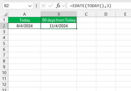
Pair THAT with the EDATE function, and you’ve got a dynamic duo capable of jumping months in a single bound. Picture this: =EDATE(TODAY(),3) in a cell, and bam – you’ve cast a glimpse three months into the future. It’s a nifty trick for forecasting and getting a heads-up on what’s looming on the financial horizon.

Turn Back Time: Calculating 90 Days before Today

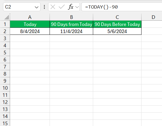
Let’s say you’re bitten by the nostalgia bug or you need real insights from the past. Sifting through old calendars is so last season. Instead, let’s harness the magic formula =TODAY()-90. All it takes is a simple cell spell casting in Excel, and voilà, you’re transported 90 days into the past.

No more fumbling with counting days or accounting for varying month lengths; Excel has got your back, ensuring leap years and those pesky February anomalies don’t trip you up. Imagine knowing what date fell 90 days before today with such ease and accuracy. Whether it’s for retrospective analysis, checking compliance deadlines, or reminiscing special dates, this formula has you covered.

Using the EDATE Function for More Complex Scenarios

The EDATE function can be useful if you need to subtract a certain number of months from a date, but it can also handle days if combined with other functions.

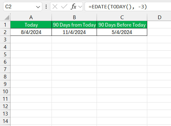
Enter the formula:

=EDATE(TODAY(), -3)

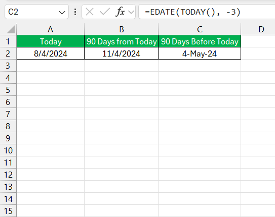
Example: If today is August 4, 2024, the formula =EDATE(TODAY(), -3) will correctly result in May 4, 2024.

 

Advanced Tricks and Tips

Format Dates in Excel

You can format the cell as a date if it’s not already formatted as such. To do this:

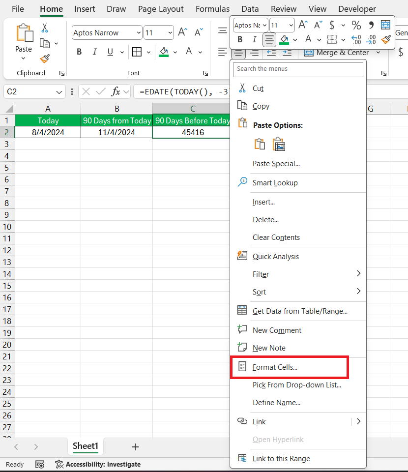
STEP 1: Right-click the cell with the formula. Choose “Format Cells.”

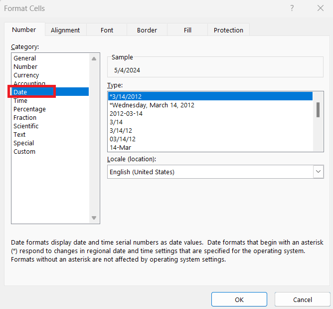
STEP 2: Select the “Date” category.

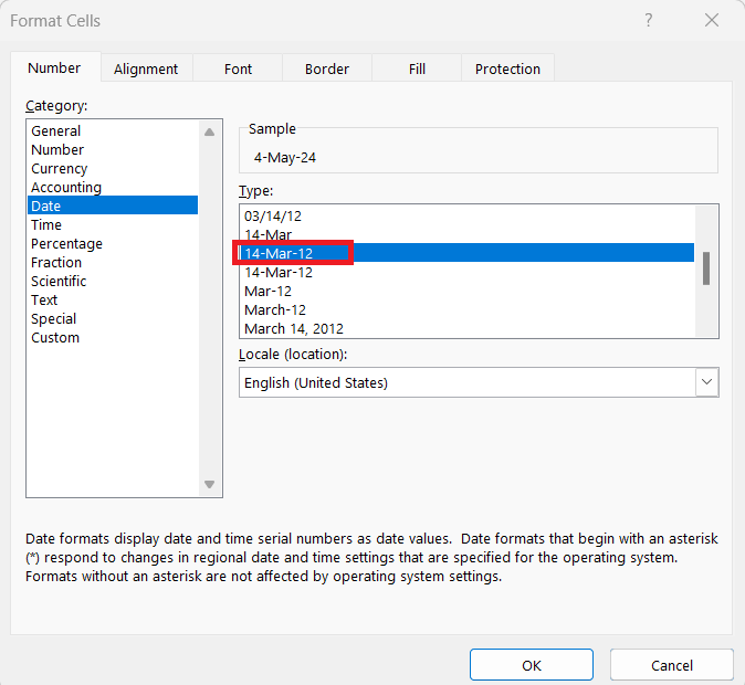
STEP 3: Choose the desired date format. Click “OK.”

The formatted date will be displayed.

 

Visual Cues: Highlighting Dates That Meet Criteria

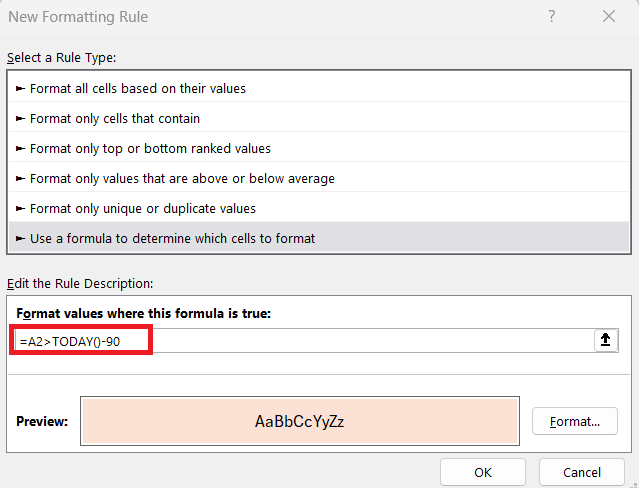
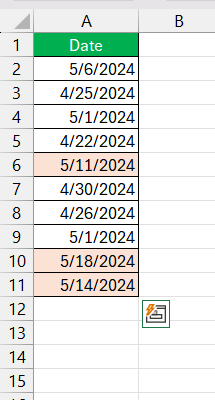
Imagine your Excel sheet not just as a data depository, but as a vibrant dashboard where important dates pop out with the urgency or calmness they deserve. Thanks to conditional formatting, you can create visual cues that instantly communicate status.

Need to spotlight dates that are closing in on the 90-day mark? No problem. Highlight the cells, tap into the Conditional Formatting tool, and craft a rule with the simple yet powerful =B2>TODAY()-90.

Voila, dates within that critical three-month window glow with your chosen hue of forewarning or encouragement.

This visual prompt brings attention to time-sensitive tasks, making sure nothing slips through the cracks of a busy schedule. It’s a matter of not just finding the data you need but actually seeing it; a truly enlightened way to interact with your spreadsheets.

 

Navigating Complications in Business Days Calculation

Defining Business Days: Exclude Weekends and Holidays

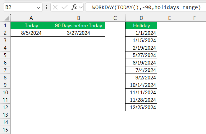
When it comes to business, not all days are created equal. Saturdays and Sundays take a backseat, and public holidays? They’re on a list all their own. Define business days in Excel by sidestepping weekends and specified holidays to get a true sense of working timelines.

By using formulas like =WORKDAY(TODAY(),-90,holidays_range), you ensure only Monday through Friday are counted, and your ‘holidays_range’ – that’s a pre-defined list of no-go dates – gets the respect they deserve.

Suddenly, calculating 90 business days before today takes into account the ebbs and flows of the corporate calendar, allowing for more accurate planning and deadline setting.

 

Frequently Asked Questions

How to calculate 90 days prior to a date in Excel?

To calculate 90 days prior to a specific date in Excel, use the formula =A1-90, where A1 is the cell containing the start date. Excel will then display the date that lands 90 days before the date you’ve provided. It’s a really straightforward process which ensures that you’re looking at the correct historical context for your needs.

How Can I Calculate Business Days Instead of Calendar Days?

To focus on business days, sidestep weekends and holidays using the WORKDAY function in Excel. Enter =WORKDAY(A1, -90, holidays_range) where A1 holds the end date, -90 represents the number of business days you’re tracking back, and ‘holidays_range’ is the named cell range containing any holidays to exclude. This way, you’ll be counting only the days when business is usually conducted.

What If I Need to Calculate 90 Business Days From a Certain Date?

If you need to calculate 90 business days from a certain date excluding weekends and any holidays, use the WORKDAY function like this: =WORKDAY(A1, 90, holidays_range), where A1 is the starting date, 90 is the number of business days, and ‘holidays_range’ is an optional list of dates to exclude, such as public holidays. This keeps your schedule on track with the actual workdays.

Are There Any Special Excel Add-ins to Simplify These Calculations?

Indeed, there are special Excel add-ins designed to simplify date calculations. Add-ins like Ablebits Date & Time Wizard offer a more user-friendly interface, allowing you to perform complex date calculations without memorizing formulas. These can be especially helpful for quickly finding deadlines, scheduling tasks, or planning events directly within your Excel workspace.

How do I conditional format in Excel for 90 days?

To conditional format in Excel for dates within 90 days, select your date cells, then navigate to ‘Conditional Formatting’ on the Home tab. Choose ‘New Rule’, and opt for ‘Use a formula to determine which cells to format’. Input the formula =AND(A1<=TODAY()+90, A1>=TODAY()) to highlight dates up to and including 90 days from today, providing a clear visual for upcoming time-sensitive items.