3 Examples to Master SUMPRODUCT in Excel

You might be familiar with the essential function like SUM and PRODUCT in Excel, but there is also a remarkable function called SUMPRODUCT. The SUMPRODUCT function in Excel is a versatile tool that empowers users to easily perform complex calculations. SUMPRODUCT in Excel returns the sum of the products of corresponding ranges or arrays. It can be used to calculate the mean salary of employees, the average score on an exam, or the mean selling price of a company’s inventory, total investment value, etc.

 

Key Takeaways:

• The `SUMPRODUCT` function in Excel is versatile and can be combined with other functions, like `ISNUMBER` and `SEARCH`, to perform complex searches within text strings. Using `SUMPRODUCT` with arrays of conditions allows users to test multiple criteria within a single cell and sum the instances where the criteria are met.
• By using `SUMPRODUCT` in combination with the double unary operator (–) to coerce TRUE/FALSE values to 1s and 0s, Excel users can create formulas that effectively count the number of times specific substrings appear within a cell. This can be particularly useful for analyzing text data and returning results that indicate the presence of certain keywords or phrases.
• Embedding `SUMPRODUCT` into the `IF` function can improve the utility and user-friendliness of Excel worksheets. Users can provide custom output rather than simple TRUE/FALSE values, which helps in creating more readable and interpretable spreadsheets, tailored to specific data analysis needs or user requirements.

 

Download the Excel Workbook below to follow along and understand how to use SUMPRODUCT in Excel – download excel workbookSUMPRODUCT-in-Excel.xlsx

 

Introduction to SUMPRODUCT in Excel

The SUMPRODUCT in Excel is a versatile tool that performs the task of calculating the total sum derived from the products of corresponding components within given ranges or arrays. The syntax of SUMPRODUCT in Excel is –

=SUMPRODUCT(array1, [array2], [array3], …)

• array1 -The first array argument whose components you want to multiply and then add. Required.
• array2, array3, … – Array arguments 2 to 255 whose components you want to multiply and then add. Optional.

Please Note – The dimensions of the arrays should be the same or else this function will return an error.

Let us look at an example to understand better.

 

#1 – Basic Example

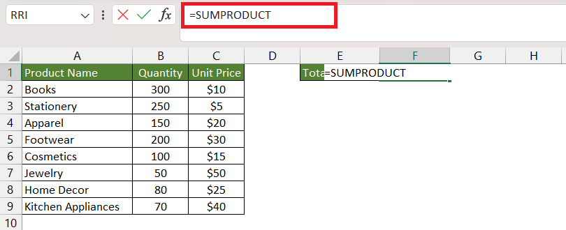
Suppose you have a dataset containing the quantities of different items sold and their respective prices. You want to calculate the total revenue generated from these sales. Here’s where SUMPRODUCT comes to your rescue.

STEP 1: Enter the SUMPRODUCT function.

=SUMPRODUCT

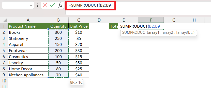
STEP 2: Enter the first argument i.e. array1. Here, it is the range containing the quantity of items sold (B2:B9).

=SUMPRODUCT(B2:B9

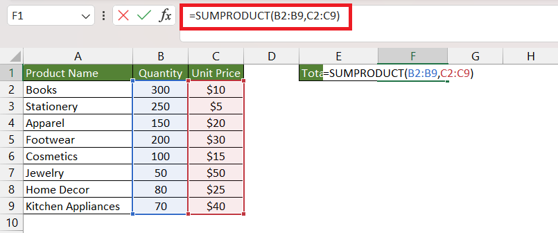
STEP 3: Enter the second argument i.e. array 2. Here, it is the range containing the unit price of the items sold (C2:C9).

=SUMPRODUCT(B2:B9,C2:C9)

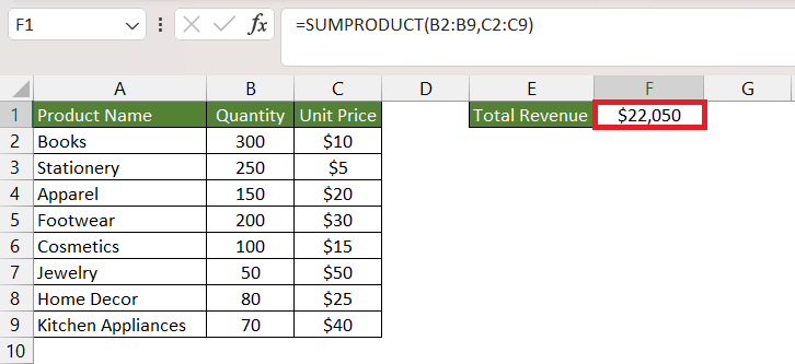
Let’s evaluate this formula –

=SUMPRODUCT(B2:9,C2:C9)

=SUMPRODUCT({300;250;150;200;100;50;80;70},{10;5;20;30;15;50;25;40}) 

=SUMPRODUCT({3000,1250,3000,6000,1500,2500,2000,2800})

=22050

Excel will first multiply each item in array1 with the corresponding item in array2 and then simply sum the result. The SUMPRODUCT function simplifies what would otherwise involve multiple steps, making it a valuable asset for straightforward calculations.

 

#2 – SUMPRODUCT with other Arithmetic Operators

While multiplication is the default operation, addition, subtraction, and division can also be applied. Utilize SUMPRODUCT in the usual manner, but instead of using commas to separate array arguments, use the desired arithmetic operators (*, /, +, -). For example, to use division with 2 arrays –

=SUMPRODUCT(array1 / array2)

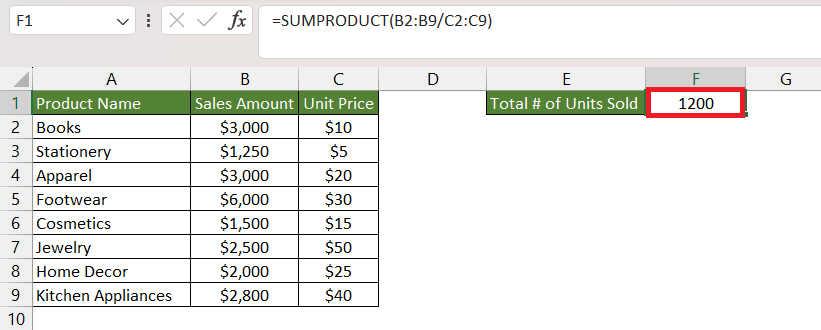
Suppose, we have a dataset with the total sales amount and unit process of different items sold. We want to know the total number of items sold based on the data provided. To do this, we need to first divide the total sales amount by the unit price for each item and then simply add the result to get the total quantity sold.

Instead, we can also use the SUMPRODUCT function by replacing the comma with the division sign to get the result –

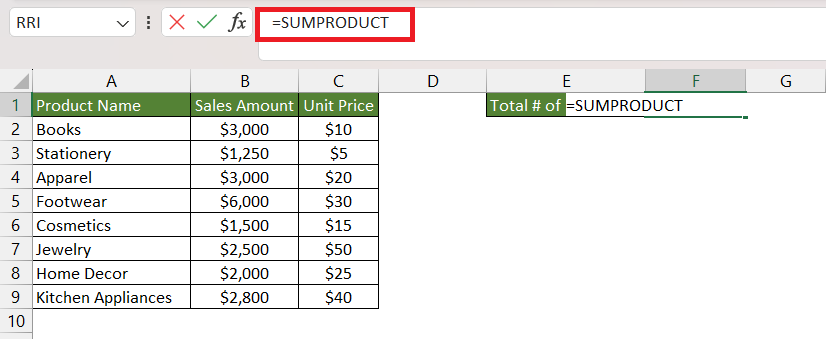
STEP 1: Enter the SUMPRODUCT function.

=SUMPRODUCT

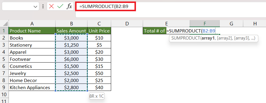
STEP 2: Enter the first argument i.e. array1. Here, it is the range containing the total sales amount (B2:B9).

=SUMPRODUCT(B2:B9

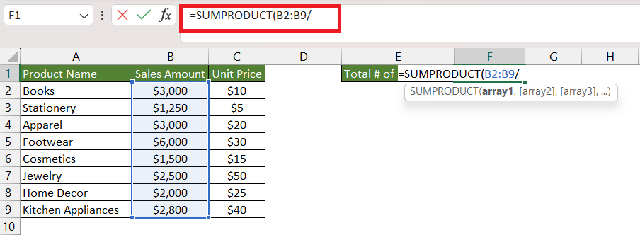
STEP 3: Enter the division operator (/).

=SUMPRODUCT(B2:B9/

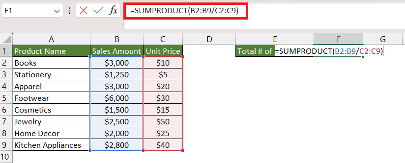
STEP 4: Enter the second argument i.e. array 2. Here, it is the range containing the unit price of the items sold (C2:C9).

=SUMPRODUCT(B2:B9/C2:C9)

=SUMPRODUCT(B2:B9/C2:C9)

=SUMPRODUCT({3000;1250;3000;6000;1500;2500;2000;2800}/{10;5;20;30;15;50;25;40})

=SUMPRODUCT({300,250,150,200,100,50,80,70})

=1200

Excel returns the total number of units sold by dividing the sales amount by the unit price and then adding the result.

 

#3 – Weighted Averages

SUMPRODUCT can also be used to calculate weighted averages in different scenarios.

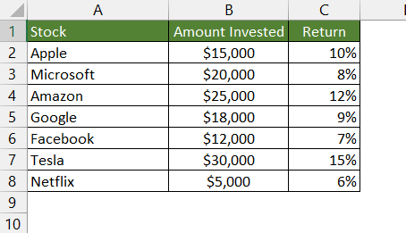
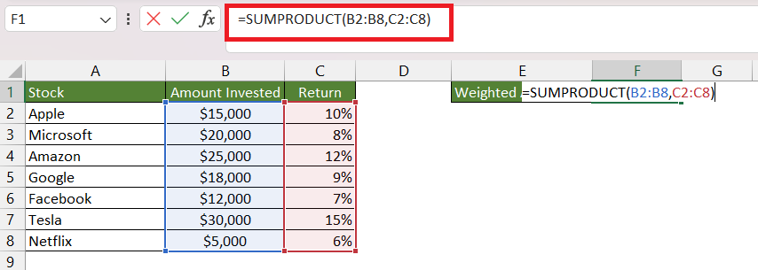
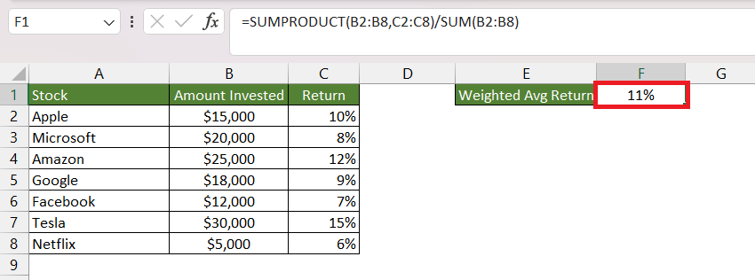
Suppose, you have invested in a portfolio of stocks, and you want to calculate the weighted average return for your investments. You have the total amount invested and the corresponding returns in percentage for all the stocks. Using the SUMPRODUCT function, you can determine the overall weighted average return of your portfolio.

You will have to first use the SUMPRODUCT function to calculate the total return (in $) of the investment by multiplying the amount invested with the return% and then adding the result. Then, you will divide this by the total investment made to get the average return of the portfolio.

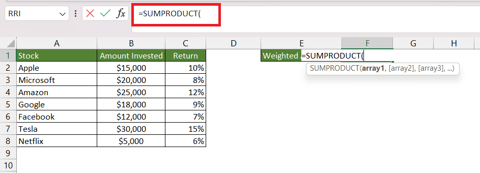
STEP 1: Enter the SUMPRODUCT function.

=SUMPRODUCT

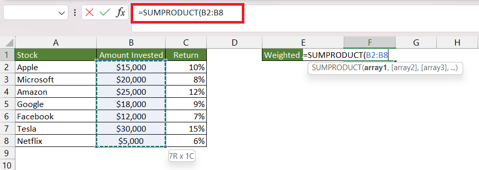
STEP 2: Enter the first argument i.e. array1. Here, it is the range containing the amount invested (B2:B8).

=SUMPRODUCT(B2:B8

STEP 3: Enter the second argument i.e. array 2. Here, it is the range containing the return of each investment made (C2:C8).

=SUMPRODUCT(B2:B8,C2:C8)

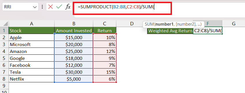
Now we have the total return, we can easily get the average return (%) by dividing it by the total amount invested.

STEP 4: Enter the division operator (/) and then the SUM function.

=SUMPRODUCT(B2:B8,C2:C8)/SUM(

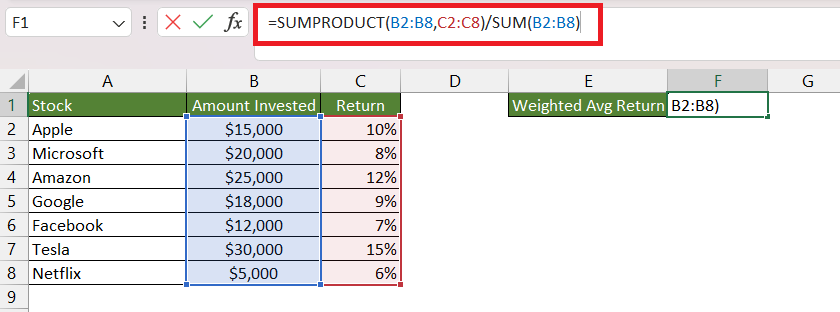
STEP 5: Select the range containing the amount invested i.e. B2:B8.

=SUMPRODUCT(B2:B8,C2:C8)/SUM(B2:B8)

Using the SUMPRODUCT and SUM functions, you can easily calculate weighted averages in any scenario.

Troubleshooting Common SUMPRODUCT Issues

Resolving the Dreaded #VALUE! Error

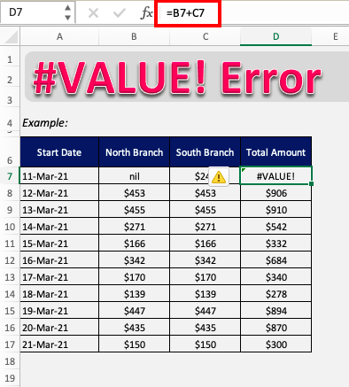
When you encounter the #VALUE! error while using SUMPRODUCT, it often means there’s a mix of text and numerical data within your selected ranges. Sometimes, this error pops up because a cell is mistakenly formatted as text, or maybe it contains a result from another formula that isn’t number-friendly. To get things back on track, make sure all cells in the range you’re working with contain numbers or are coercible to numbers. You’ll be surprised how often checking the data type resolves your issue!

Debugging SUMPRODUCT Syntax Problems

Tackling syntax issues in SUMPRODUCT can be a bit like solving a puzzle. First and foremost, remember that your ranges need to match in size. If they don’t, SUMPRODUCT will gift you an error because it cannot pair the corresponding elements. Next, look out for misplaced parentheses which can throw your formula off balance. Each argument should be correctly enclosed to ensure that the function can read and process your data accurately.

Keep an eye on operators as well. If you’ve decided to add some mathematical flair to your formula by incorporating addition or subtraction, confirm that these operators are not causing conflicts by being in the wrong place. A clear and correctly structured formula not only runs smoothly but is also easier for anyone else peering into your workbook to understand and maintain.

Best Practices and Tips for Efficient Usage

Understanding Array1, Array2 Notation

Diving into SUMPRODUCT without understanding the notation is like trying to read a map without knowing the symbols. Luckily, it’s quite straightforward once you get the hang of it. Array1 refers to the first group of values you want to multiply together. This is your starting point, containing the set of multiplicands that SUMPRODUCT will first bear down on.

Then, Array2 (and any subsequent arrays like Array3, Array4, etc.) joins the party as optional guests. You can summon them when you need to multiply corresponding items across multiple ranges. Think of these arrays as additional layers of data that SUMPRODUCT will iterate over, multiplying and then adding their products to the grand total.

In other words, Array1 is the non-negotiable invitee to your SUMPRODUCT formula shindig, and Array2 and beyond are plus-ones, there to jazz things up when conditions call for it. Embrace the notation, and you’ll unlock a new world of calculation capability in Excel.

Keeping it Quick and Clean with SUMPRODUCT

Maintaining speed and efficiency in your Excel workbooks is paramount, especially when you’re dealing with sizable data sets. With SUMPRODUCT, the aim is to keep things zippy and tidy. You can speed things up by using named ranges to refer to your data. This not only makes your formulas easier to read but also reduces the chance of referencing errors.

Secondly, avoid using entire column references in your SUMPRODUCT formula. While it might be tempting to simply use ‘B:B’ instead of ‘B1:B100’, this can lead to slower calculation times as Excel works through tens of thousands of unnecessary cells. Instead, be specific with your range—a practice that’ll keep your workbook working at its snappiest.

Also, remember that keeping formulas direct and to the point aids in preserving workbook cleanliness. If you can do something elegantly with one SUMPRODUCT formula, there’s rarely a need to bloat your workbook with several more complicated operations.

FAQs: Your SUMPRODUCT Questions Answered

Why Use SUMPRODUCT Over Other Sum Functions?

SUMPRODUCT is your go-to for versatility and strength in calculations. Unlike other sum functions that might hit a roadblock with certain conditions or require setting up multiple intermediary steps, SUMPRODUCT extends beyond just adding numbers—it multiplies corresponding elements across arrays and then sums up those products. This unique ability means you can perform complex formulas in a one-liner, where others like SUM or SUMIF might need additional help or simply can’t cope.

Moreover, because SUMPRODUCT doesn’t require array-entered formulas, you can avoid the cumbersome Control + Shift + Enter process, streamlining your Excel experience even more. If you cherish a clean spreadsheet and appreciate efficiency, SUMPRODUCT has got your back.

Can SUMPRODUCT Handle OR Logic Successfully?

Absolutely, and that’s one of the highlights of using SUMPRODUCT – it’s quite the multitasker when it comes to applying logic conditions! SUMPRODUCT can effortlessly process OR logic within your criteria, which sets it apart from its siblings SUMIFS and COUNTIFS, which strictly adhere to AND logic.

To work in that OR logic, you would utilize the plus operator (+) to include multiple conditions. Think of it as telling SUMPRODUCT, “Hey, sum the total values if this OR that criterion is met.” The function then diligently follows through, summing up the values when either of the given conditions holds true.

So if you ever find yourself needing to sum across diverse conditions without writing a total saga of separate formulas, remember that SUMPRODUCT can manage OR logic nimbly, simplifying your spreadsheet life.

How to Adapt SUMPRODUCT for Counting Unique Occurrences?

Counting unique occurrences may not be what SUMPRODUCT is known for, but with a few tweaks, it’s certainly up to the challenge. Adapt SUMPRODUCT for this purpose by combining it with other functions like COUNTIF. Essentially, you’ll be setting up a formula that inversely weights repeated items, so if an item appears more than once, it contributes less to the final count.

A formula might look something like this: =SUMPRODUCT(1/COUNTIF(range, range)), which cleverly ensures that each unique item is counted once. The COUNTIF part calculates how many times an item appears within the range, and then SUMPRODUCT sums up the reciprocals of those counts — effectively counting each distinct item just once.

Remember, this nifty transformation is especially useful if you’re working with a version of Excel that doesn’t support the UNIQUE function. Using SUMPRODUCT in this way to count unique occurrences illustrates just how much of a Swiss Army knife it can be in your Excel toolset.

SUMPRODUCT calculates the sum of products of corresponding elements within given arrays or ranges. This function finds application in various scenarios, including basic calculations like total revenue from sales, complex operations involving different arithmetic operators, and calculating weighted averages, such as determining the weighted average return on investments in a diverse portfolio.