Ascending in Excel: Fast Sorting with Formulas & Functions

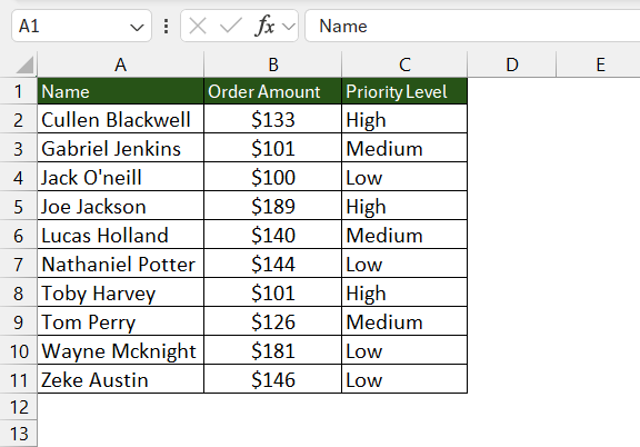
This article unveils the essential role of sorting in managing and analyzing data within Microsoft Excel. It highlights how sorting transforms data chaos into order, enhancing clarity and accuracy for better decision-making. Through ascending sorts, custom formulas, and addressing common pitfalls, the article guides readers from basic techniques to advanced sorting strategies, empowering them with the skills to navigate Excel’s sorting functionalities efficiently.

Key Takeaways

• Utilizing ascending sort in Excel organizes data from smallest to largest, aiding in trend identification and data preparation for further analysis.
• Developing custom formulas allows for tailored sorting based on specific needs, offering flexibility for complex or unique datasets.
• Recognizing and addressing common sorting issues, such as hidden characters or merged cells, is crucial for maintaining data integrity during sorting operations.
• Excel’s advanced sorting functions, like SORT and SORTBY, automate and refine data organization, saving time and enhancing analytical efficiency.

Download the spreadsheet and follow along with the blog on How to sort data in ascending in Excel – Download excel workbookAscending-in-Excel.xlsx

 

Sorting to Simplicity

The Power of Organizing Data in Excel

Excel is more than just a spreadsheet application; it’s a powerful tool that can help you manage and analyze vast amounts of data. Whether you’re juggling financial records, managing inventory, or tracking projects, Excel’s sorting capabilities assist in bringing order to chaos. By efficiently arranging data, you increase both clarity and accuracy in your analysis, leading to more informed decision-making.

Ascending Sort: A Path to Clarity

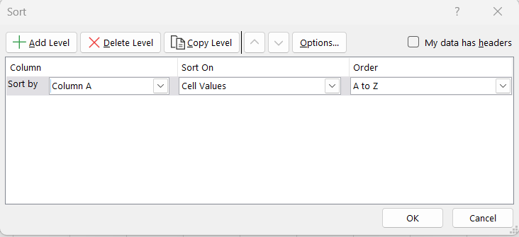
Ascending sort is like your data’s GPS, guiding each piece of information to its rightful place in the grand scheme of your spreadsheet. Select your dataset, then click on the ‘Sort’ button in the ‘Data’ tab.

When the Sort dialog box appears, choose your first column under ‘Sort by’, set ‘Sort On’ to ‘Cell Values’, and ‘Order’ to A to Z for ascending sort.

This method ranks your data from the smallest value to the largest, whether that’s A to Z or 1 to 10, ensuring that patterns and insights emerge naturally from your dataset. It’s essential for preparing data for further analysis, whether you’re looking to identify trends, streamline processes, or simply make your data more digestible.

 

Quick Guide to Sorting with Formulas

Creating custom formulas to sort in Excel is like tailoring a bespoke suit—it’s all about the perfect fit for your unique data’s needs. While pre-built functions are handy, sometimes they may lack the flexibility required for complex or non-standard data sets.

That’s where crafting a formula comes into play, enabling you to sort based on multiple criteria, incorporate conditional logic, or handle errors more gracefully. This approach empowers you with granular control over how your data is ordered, making it possible to uncover the exact insights you’re searching for.

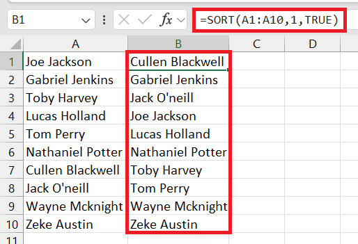
• Basic numeric sort formula: =SORT(A1:A10,1,TRUE)

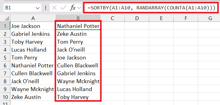
• Random sort formula: =SORTBY(A1:A10, RANDARRAY(COUNTA(A1:A10)))

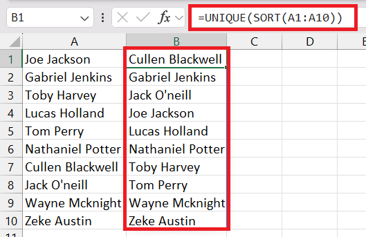
• Sort and extract unique values: =UNIQUE(SORT(A1:A10))

Advancements in Excel Sorting

Overcome Common Sorting Pitfalls

Navigating through sorting in Excel can sometimes feel like an obstacle course, but with the right know-how, you can easily jump over common pitfalls. A frequent hurdle is when data isn’t sorted as expected, which can happen if there are hidden characters, inconsistent data types, or merged cells disrupting the sort sequence.

Another issue is partial sorting, where only a portion of the table is sorted, breaking data associations across rows. By ensuring a consistent data structure and unmerging cells before sorting, you can maintain data integrity and achieve a flawless sort every time. It’s also wise to employ filter criteria and clearly label headers to avoid confusion and unintended results.

• Double-check data types for consistency.
• Unmerge cells and remove any hidden characters.
• Use Data Validation to maintain data integrity.
• Ensure the entire dataset is selected prior to sorting.
• Apply filters to avoid sorting unwanted data sections.

 

Understand and Fix #SPILL, #REF, and #VALUE Errors in Sorting

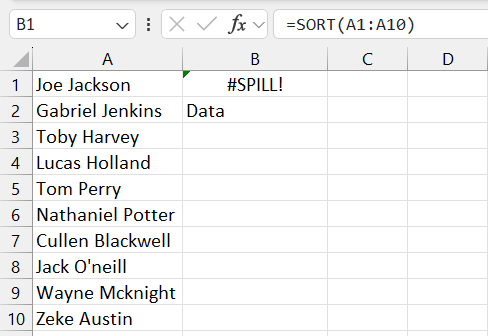
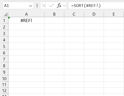
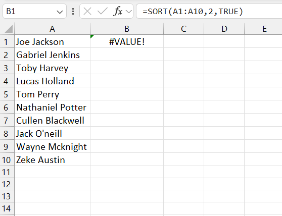
To keep your data flowing smoothly without spillages, it’s crucial to understand the #SPILL error and its companions, #REF and #VALUE. The #SPILL error often occurs when there’s not enough space for a formula to display all its results, whereas #REF errors pop up when a formula references a cell that’s not there anymore. Meanwhile, the #VALUE error can sneak in if your formula is expecting a number but gets text instead, or if there are other argument mismatches.

Here’s how to troubleshoot these errors in your sorting adventures:

• #SPILL Error: Ensure no cells are blocking the range where data is expected to spill. Look for and eliminate merged cells or pre-existing data in adjacent cells.

• #REF Error: Check your formula for invalid cell references. This often happens when cells are deleted or cut.

• #VALUE Error: For sorting, ensure your sort_index doesn’t exceed the number of columns. Also, double-check that your sort_order is either 1 for ascending or -1 for descending.

 

By vigilantly avoiding cell blockages and argument mismatches, you’ll clear the path for error-free, ascending sort actions.

 

Sorting Beyond Numbers

Custom Sorting Options in Excel

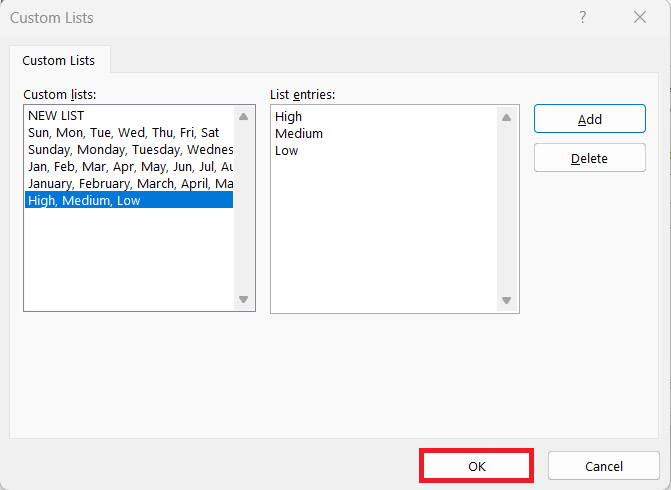
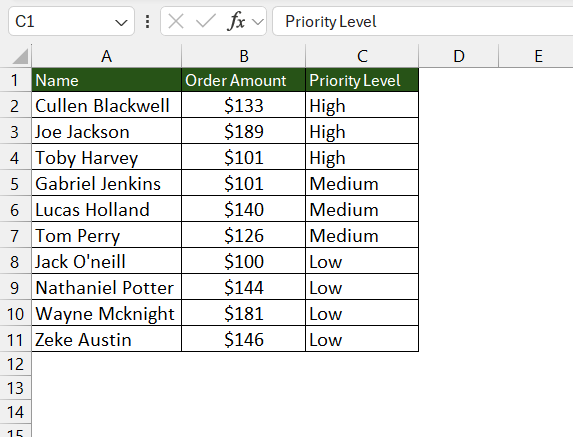
Custom sorting in Excel is your go-to when the standard A-Z or 1-10 order just doesn’t cut it. It’s like putting together a puzzle where you define the final picture. You can create a specific sort order tailored to your dataset needs, like prioritizing certain rows or establishing an unconventional order (such as t-shirt sizes or levels of urgency). Excel’s custom lists are particularly useful for times when the default sorting options are not adequate to capture the nuances of your real-world data.

To get started with custom sorting:

STEP 1: Select your dataset and click on the ‘Sort’ option in the Data tab.

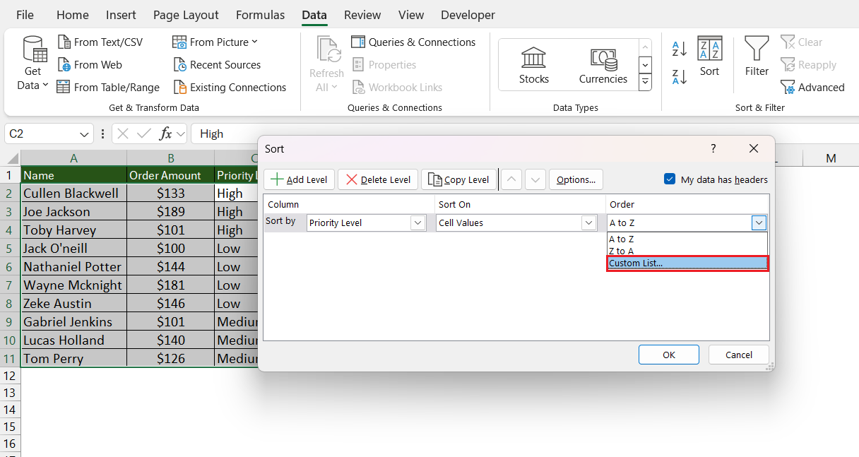
STEP 2: Ascending in Excel Fast Sorting with Formulas Functions – Choose the column to sort by and select ‘Custom List’ from the ‘Order’ dropdown.

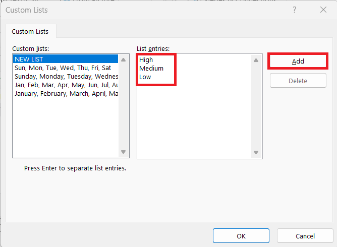
STEP 3: In the Custom Lists dialog box, enter your list entries in the desired sort order. Click ‘Add’.

STEP 4: Click ‘OK’ to apply your custom sort order.

The data will be sorted as per the custom list provided.

This feature is especially helpful when dealing with categorical data that requires a specific hierarchy.

 

Manipulating Text and Dates with Sorting Techniques

Mastering the art of sorting in Excel extends beyond simple number columns; you can also deftly manipulate text and dates to align with your objectives. Imagine you have a list of names that you want to see alphabetically or a series of events that you want to chronologically organize; sort functions can be tailored to manage these data types proficiently.

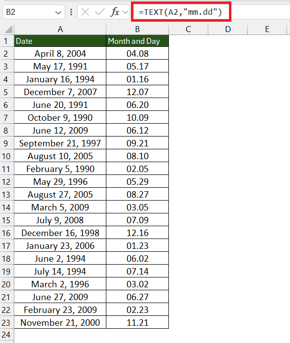
With text data, you have the option to sort in alphabetical order or even use functions like LEFT, MID, and RIGHT to sort based on specific characters within the cells. For dates, Excel recognizes them as serial numbers, allowing you to sort them chronologically. Plus, with formulas like TEXT and DATE, you can sort birthdays, anniversaries, and other recurring events by day and month, regardless of the year.

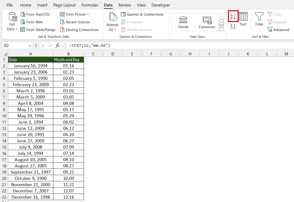
For example, you can organize birthdays using the formula: =TEXT(B2, "mm.dd") Then, sort the results to get a clear view of upcoming celebrations, neatly organized by month and day.

Go to the Data tab and select A to Z.

Be it planning schedules, prioritizing tasks, or simply making sense of a jumbled list, these sorting techniques have you covered.

 

Sort Like a Pro

Excel Table Tricks for Auto-Expanding Sorts

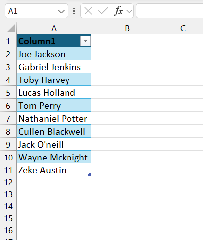
Excel tables offer a secret superpower: auto-expanding sorts. When setting up a table, any added data automatically becomes a part of the dynamic range. Say goodbye to manually adjusting your data selection every time new information is added – Excel tables handle this gracefully.

Here’s a trick to leverage Excel tables for hassle-free sorting:

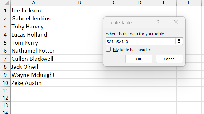
STEP 1: Convert your data range into a table by selecting it and pressing Ctrl + T.

STEP 2: Ensure that the ‘My table has headers’ option is checked to properly set up your columns.

As you input new data, the table will expand, including these entries in your sorted lists without you lifting a finger.

When sorting a table, the sorting state is preserved, meaning that even if data is added or changed, clicking anywhere within the table and sorting again will maintain the order you’ve applied, reflecting the new data consistently.

 

Dealing with Multi-Level and Multi-Column Sorting Challenges

Multi-level and multi-column sorting in Excel allows you to finesse your way through complex datasets, creating a hierarchy of sort conditions that reflect the multi-faceted nature of your data. This can be particularly useful when working with extensive lists where a single sort criterion doesn’t provide the clarity needed.

To effectively tackle this challenge:

STEP 1: Click on the Sort option within the Data tab while your dataset is selected.

STEP 2: Start with your primary sort key by selecting the column and choosing the sort order.

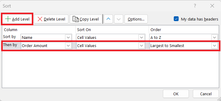
STEP 3: Use the ‘Add Level’ feature to include additional sort criteria, arranging them in the order of their sorting priority.

STEP 4: Repeat step 3 as necessary for multiple levels, and then apply the sort to organize your data across multiple columns.

The data will be sorted as per the levels mentioned.

Remember: the sequence in which you apply these levels is crucial — Excel will sort data based on the first criterion, then the second, and so forth, in a nesting fashion.

 

Save Time with Tips and Shortcuts for Sorting Data

Efficiency is key when dealing with large datasets in Excel. To streamline your data sorting tasks, there’s a wealth of tips and keyboard shortcuts at your disposal.

Here are some time-saving tactics:

1. Quick Sort Shortcuts: Instead of navigating menus, use Alt + D + S to open the Sort dialogue box quickly, or Ctrl + Shift + L to toggle filters on and off for sorting with headers.
2. Data Selection Tip: Click on a single cell within your data before sorting to avoid Excel extending the selection incorrectly.
3. Multiple Column Sort: Hold down the Shift key while selecting additional column headers to sort by multiple columns simultaneously.
4. Persist Sort Options: Use custom sort options and save your search; next time, Excel will remember your preferences.
5. Flash Fill Feature: If you’re manually creating data based on patterns, use the Flash Fill (Ctrl + E) to have Excel recognize the pattern and auto-fill the rest for you.

By incorporating these shortcuts into your routine, you’ll notice immediate gains in your sorting tasks – reducing what used to take minutes into mere seconds.

 

FAQs

What is the Basic Formula for an Ascending Sort in Excel?

The basic formula for an ascending sort in Excel is the SORT function, which looks like this: =SORT(range, [sort_index], [sort_order], [by_col]). If you want to sort a single column in ascending order, you’d simply specify the range and leave the other parameters at their defaults. For example, =SORT(A2:A100) would sort the range A2 through A100 in ascending order.

How Do I Sort Multiple Columns in Ascending Order in Excel?

To sort multiple columns in ascending order in Excel, first select your dataset, then click on the ‘Sort’ button in the ‘Data’ tab. When the Sort dialog box appears, choose your first column under ‘Sort by’, set ‘Sort On’ to ‘Cell Values’, and ‘Order’ to A to Z for ascending sort. To add another column, click ‘Add Level’, choose your second column, repeat the sorting preference, and continue this process for any additional columns you wish to sort in ascending order.

What is the shortcut for ascending numbers in Excel?

To sort numbers in ascending order using a shortcut in Excel, first select the range or column you wish to sort. After selecting, you can use the Alt + D + S shortcut which brings up the Sort dialog box. Then you can specify your sort criteria and ensure that the ‘Order’ is set to ‘Smallest to Largest’ before confirming your sort operation.

How to arrange numbers in descending order in excel using formulas?

To arrange numbers in descending order in Excel using formulas, use the LARGE function in combination with ROW or the SORT function. For example, to sort a column of numbers, you’d use =SORT(A2:A100, 1, FALSE), where FALSE specifies descending order. With the LARGE function, if you’re looking for the largest value in a range, you would use =LARGE(A2:A100, ROW(1:1)), and drag the formula down to get subsequent values in descending order.

What if you only want to return a specific sort position?

If you only need to return a specific sort position from an Excel range, you can use the INDEX combined with SORT like so: =INDEX(SORT(range, sort_index, sort_order), position). For example, to return the value from the first position in a list sorted in descending order, use =INDEX(SORT(A2:A100, 1, FALSE), 1). You can change the position number to get the 2nd, 3rd, or any specific sorted position you require.