How to Find the Average Value with Excel Formulas

Calculating averages is a fundamental aspect of data analysis, and Excel makes this task straightforward with its built-in functions. In this article, I’ll show you how to find average value using Excel’s powerful tools, helping you make sense of your data quickly and efficiently. Whether you’re working with simple datasets or more complex information, mastering average calculations can provide valuable insights and streamline your data management.

Key Takeaways:

• The AVERAGE Function: The AVERAGE function in Excel simplifies calculating the arithmetic mean of a dataset, making data analysis quicker and easier.
• Basic Syntax and Usage: To use the AVERAGE function, enter =AVERAGE(range) where “range” is the group of cells containing the data you want to average.
• Advanced Functions: Utilize AVERAGEIF for conditional averaging and AVERAGEIFS for multiple criteria to gain more nuanced insights from your data.
• Handling Errors: Use IFERROR with AVERAGE to manage errors in your dataset and ensure accurate results even with problematic data.
• Excluding Unwanted Data: To refine your averages, use AVERAGEIF to exclude zeros or specific values, and ensure non-numeric data doesn’t distort your results.

 

Introduction to Excel Averaging Formulas

The Power of the AVERAGE Value

As I explore the capabilities of Excel, the AVERAGE function stands out as a cornerstone for statistical analysis. It simplifies the process of calculating the arithmetic mean—a task that can be tedious if done manually.

By quickly analyzing a set of numbers to find their central value, this function becomes indispensable in various scenarios, particularly for those in fields where data interpretation is key.

Why Mastering Average Calculation is Essential

Mastering average calculation in Excel is no mere academic exercise; it’s a practical skill that equips us to transform raw data into meaningful insights. Averages help us identify trends, understand central tendencies within datasets, and make informed decisions.

In the worlds of business, education, and beyond, these calculations serve as the backbone for performance analysis, forecasting, and strategic planning. Being adept at calculating averages means we can better gauge progress, pinpoint areas needing improvement, and celebrate success where it’s due.

 

Understanding the Basics of Excel’s AVERAGE Function

Syntax and Parameters

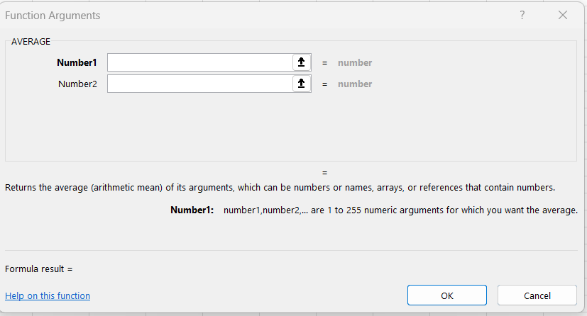
The syntax of the AVERAGE function is straightforward. It follows the pattern: =AVERAGE(number1, [number2], …). Here,

• number1 is required and represents the first number or range that you wish to include in your average calculation.
• [number2] is optional and represents additional numbers or ranges to include in the average calculation.

While number1 is a required argument, you can include up to 254 additional numbers or ranges as optional arguments. This flexibility allows you to calculate the average of large data sets efficiently.

By mastering the AVERAGE function’s syntax and parameters, we gain an invaluable tool for analyzing and interpreting data.

Using AVERAGE in Simple Calculations

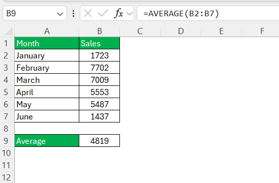
When it comes to simple calculations, using the AVERAGE function in Excel is as uncomplicated as it gets. By typing =AVERAGE( and then select the range of cells containing the data you want to average, Excel does the heavy lifting.

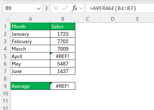
For instance, if you aim to find the average sales from January to June, you can select the cells from B2 to B7, close the parenthesis, and press Enter. The resultant figure reflects the average sales over that six-month period.

Here’s what you’d actually type into Excel: =AVERAGE(B2:B7)

This approach is not only intuitive but ensures that our data analyses are both swift and precise, freeing up our time to focus on interpreting results and making data-driven decisions.

 

Diving Deeper: Variations of the AVERAGE Function

AVERAGEIF for Conditional Averages

The AVERAGEIF function takes our data analysis a step further by allowing us to calculate averages that meet a specific condition we set. This is particularly useful when we need to pinpoint average values within a subset of our dataset. The syntax is

=AVERAGEIF(range, criteria, [average_range]),

where range refers to the cells that will be evaluated by the criteria, and [average_range] contains the actual numbers to average—if different from range.

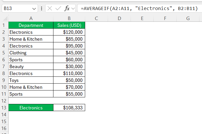
Suppose we have a list of different departments with their respective sales, and we only want to know the average sales of the ‘Electronics’ department. We could set the range to the department names, the criteria to “Electronics”, and the average_range to the sales figures.

This would look something like: =AVERAGEIF(A2:A11, "Electronics", B2:B11)

By harnessing the AVERAGEIF function, we can sift through data to find averages that are not just broad strokes but finely detailed insights tailored to very specific segments of our data.

AVERAGEIFS for Multiple Criteria

With the AVERAGEIFS function, we’re not limited to just one condition; we can calculate averages based on multiple criteria. The function becomes a powerhouse when we’re working with complex datasets where multiple factors must be considered simultaneously.

The syntax is =AVERAGEIFS(average_range, criteria_range1, criteria1, [criteria_range2, criteria2], ...), meaning we can have multiple pairs of criteria and their corresponding ranges.

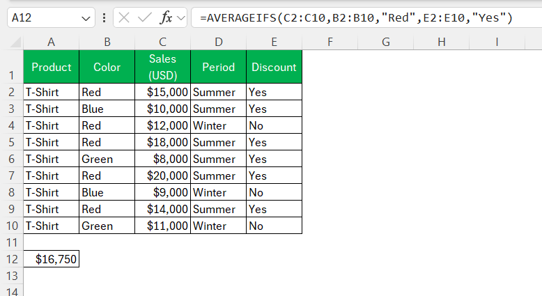
For example, imagine we want to find the average sales of red shirts sold during a summer discount period. We’d specify one condition to be the color “Red” and another to be the “Discount” period. With AVERAGEIFS, we’d do this:

=AVERAGEIFS(sales_range, color_range, "Red", discount_range, "Yes").

This would give us a precise average we’re looking for, informed by two distinct conditions.

By mastering AVERAGEIFS, we’re equipping ourselves to delve into data in a much more specific and insightful way, giving us the ability to provide nuanced analysis that is both relevant and highly targeted.

 

Common Challenges and Solutions with Averaging in Excel

Dealing with Errors During Averaging

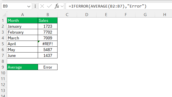
Errors can be a common stumbling block when calculating averages in Excel. When they appear in our dataset, the AVERAGE function will return an error, rather than a useful result. To circumvent this issue, we can employ the IFERROR function in conjunction with AVERAGE to filter out those pesky errors. The syntax for this workaround looks like: =AVERAGE(IFERROR(range, "")).

In practice, if we’re analyzing a range from B2 to B7 that contains some error values, we wrap our range with the IFERROR function to smoothly bypass them, like so: =AVERAGE(IFERROR(B2:B7, "Error")).

By using this error-handling strategy, we can ensure that our averaging calculations remain robust and accurate, even when the data we’re working with isn’t perfectly clean.

Excluding Zeros and Non-Numeric Data

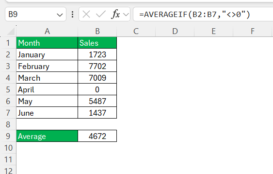
When working with ranges in Excel that include zeros or non-numeric data, we have to be cautious to ensure they don’t skew our average calculations. The AVERAGE function doesn’t account for this—it will treat zeros as valid numbers, and in doing so, may give us an inaccurate picture.

To exclude zeros, we can use AVERAGEIF or AVERAGEIFS with the criteria set to “<>0”, which translates to “not equal to zero”. This ensures that our average only takes into account non-zero numbers. For example: =AVERAGEIF(B2:B7, "<>0") gives us the average while ignoring any zeros.

To bypass non-numeric data, these functions automatically skip over text and empty cells. However, if non-numeric data is formatted as numbers or if there are error values, these will result in errors. For error values, the IFERROR function, as previously mentioned, can be employed to maintain the integrity of our dataset.

By tailoring the function we use to calculate averages, we ensure that our results are reflective of the genuine trends and patterns within our data, without distortion by unwanted zeros and non-numeric values.

 

Frequently Asked Questions

How to average function in Excel?

To use the average function in Excel, enter =AVERAGE( followed by the cells or range you want to find the average for, and then close the bracket. For instance, to average cells A1 to A5, your formula will be =AVERAGE(A1:A5). Hit Enter, and Excel calculates the average for you.

How Do I Fix the #DIV/0 Error When Averaging?

Fix the #DIV/0 error that occurs during averaging by ensuring that there is at least one numeric value in the range. Use =IF(COUNT(range)>0, AVERAGE(range), "") to return an average if the count of numbers is greater than zero, otherwise an empty string. This prevents the division by zero error.

Can I Use the AVERAGE Function to Average Times or Dates?

Yes, the AVERAGE function can average times or dates in Excel. Ensure the cells are formatted correctly as date or time. For example, =AVERAGE(range) on a range of cells with time values will give you the average time. Apply an appropriate time format to see it correctly.

How Can I Exclude Specific Values from the Average Calculation?

To exclude specific values from an average calculation, use the AVERAGEIF or AVERAGEIFS functions. For example: =AVERAGEIF(A1:A10, "<>5") will average the numbers in A1:A10, excluding any cells with the value of 5.

Is There a Way to Calculate the Average If Cells Contain Text?

To calculate an average in a range that includes text, use the AVERAGEA function, which counts text as zero. For instance, =AVERAGEA(A1:A10) will average the numeric values in the cells A1 through A10 while treating text entries as zeroes in the calculation.