Case Insensitive Filtering Using Power Query or Get & Transform

Power Query or Get & Transform (In Excel 2016) lets you perform a series of steps to transform your Excel data.  Did you know that you can do case insensitive filtering? I will show you how to do it step by step below!

Key Takeaways

• Power Query Is Case Sensitive by Default – Filtering in Power Query distinguishes between uppercase and lowercase unless explicitly handled otherwise.

• Use Text.Lower or Text.Upper for Normalization – Convert both the column values and the filter criteria to the same case (lower or upper) for case-insensitive filtering.

• Custom Columns Make Filtering Flexible – Create a custom column that transforms text using Text.Lower([ColumnName]), then filter on that.

• Great for Cleaning Inconsistent Data – Useful when working with datasets where names, categories, or labels are typed with mixed cases.

• Works Across Steps and Queries – You can apply case-insensitive logic across merged queries, grouped data, and filtered lists for accurate results.

Case Insensitive Filtering Using Power Query or Get & Transform

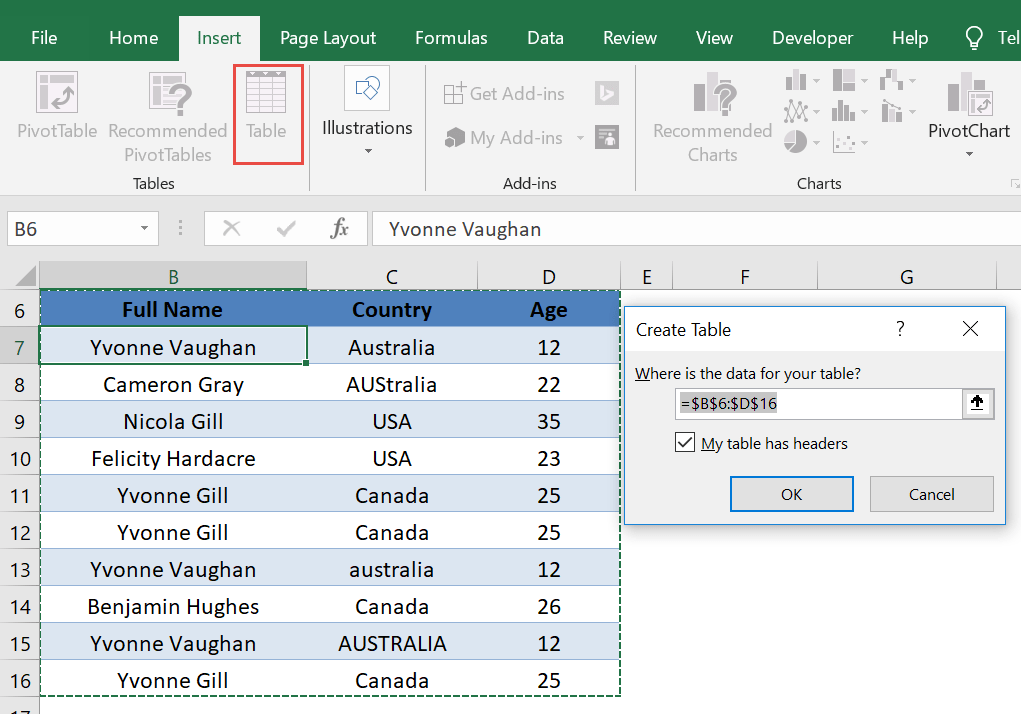
STEP 1: Select your data and turn it into an Excel Table by pressing the shortcut Ctrl + T or by going to Insert > Table

 

STEP 2: Go to Data > Get & Transform > From Table (Excel 2016) or Power Query > Excel Data > From Table (Excel 2013 & 2010)

Excel 2016:

 

Excel 2013 & 2010:

 

STEP 3: This will open up the Power Query Editor.

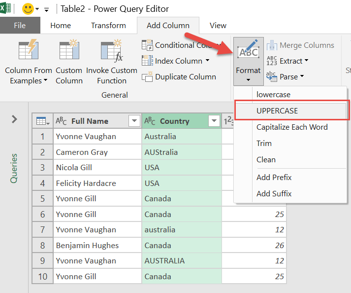
We want to filter out Australia in the Country column, however it has different capitalizations so it is difficult to filter them in one go. What do we need to do?

Let us add a new column! Ensure the Country column is selected.

Go to Add Column > From Text > Format > Uppercase

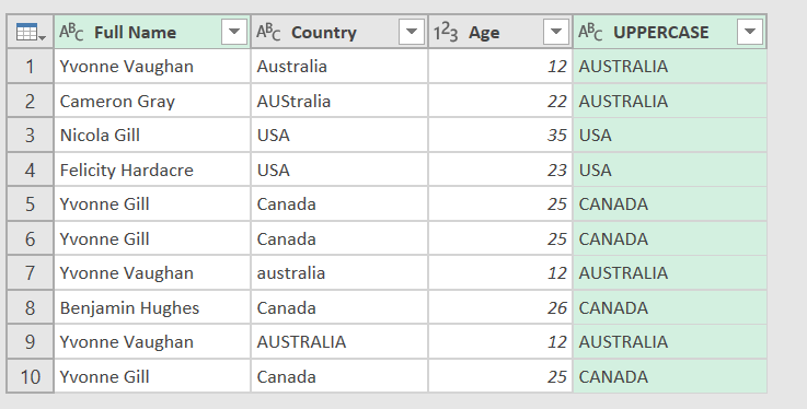
Now this should make filtering a cinch! Since all values are now AUSTRALIA:

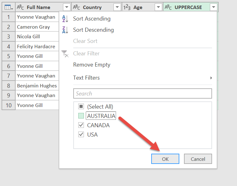
STEP 4: Now click the down arrow of your new Uppercase column and ensure Australia is unticked. Click OK.

 

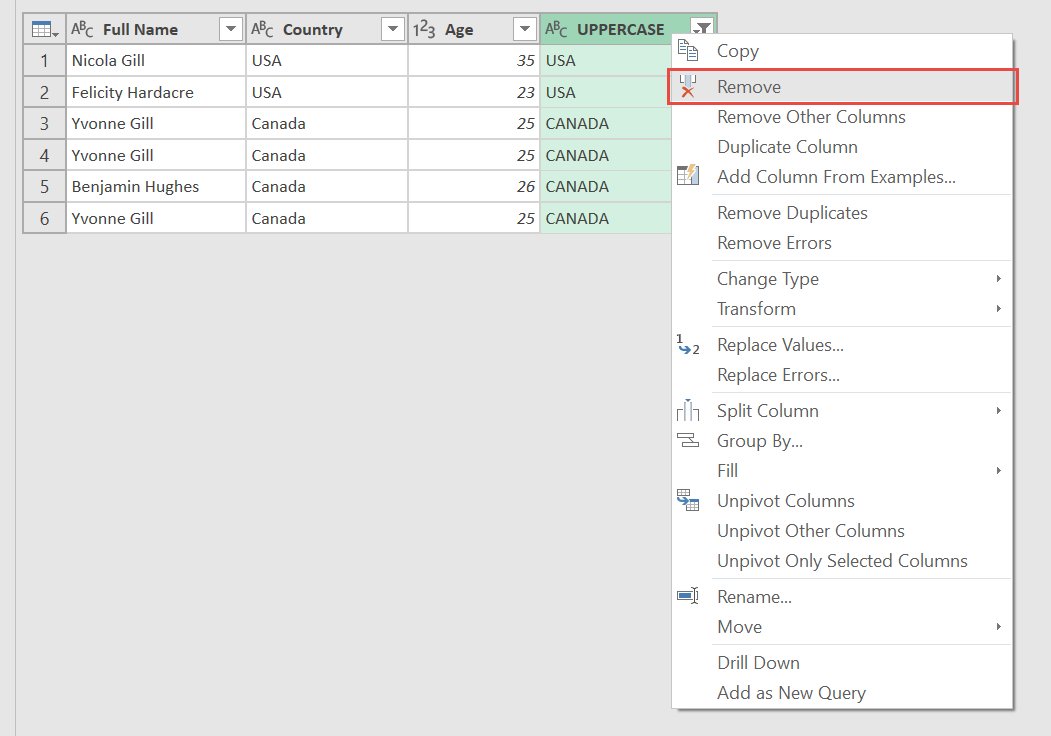
STEP 5: We do not need this column anymore, right click on the column and select Remove.

 

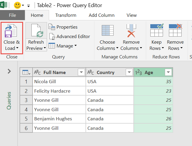
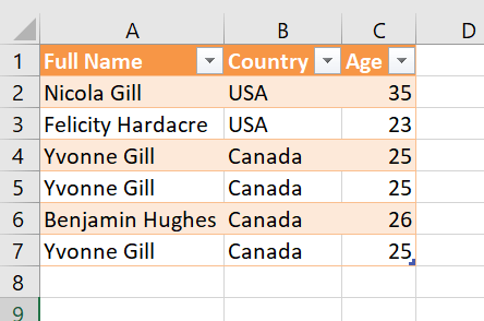
STEP 6: Click Close & Load from the Home tab and this will open up a brand new worksheet in your Excel workbook with the updated records!

You now have done your case insensitive filtering!

Frequently Asked Questions

Is Power Query case sensitive when filtering text?
Yes, by default, Power Query treats "Apple" and "apple" as different values when filtering text.

How can I perform case-insensitive filtering in Power Query?
Use the Text.Lower() or Text.Upper() function in a custom column, then filter based on the converted values.

Can I apply case-insensitive filters without adding a custom column?
You can also use Text.Lower([Column]) = "value" in the formula bar as a filter condition, but a custom column is often clearer and more reusable.

What if I’m combining data from multiple sources with inconsistent casing?
Normalize all text fields using Text.Lower() or Text.Upper() before merging or filtering for consistent, reliable results.

Does case-insensitive filtering affect performance?
The performance impact is minimal for most datasets, and it’s a recommended practice for cleaning inconsistent text entries.