Change Layout of Report Filter

At first, when I used that, I thought the layout is completely fixed. And nothing could be further from the truth! There are options that allow you to customize the report filter layout.

 

Download the workbook below to follow along with the tutorial on how to change layout of Report Filters in Pivot Table:

---

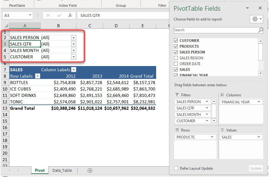
Here is our Pivot Table and you can see the layout of our filters:

 

Method 1: Switch to Horizontal List

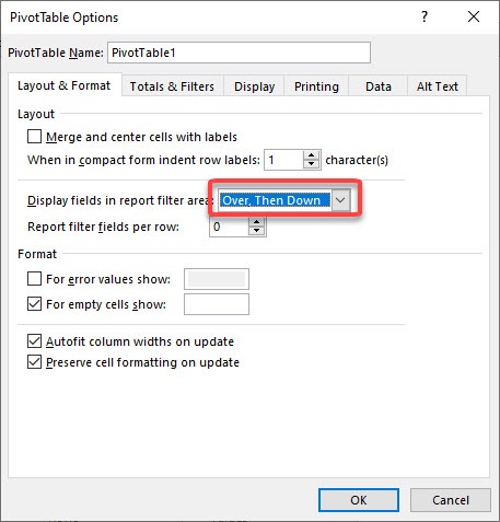
STEP 1: Let us change that! Go to PivotTable Analyze > PivotTable > Options

STEP 2: Select Over, Then Down, and click OK

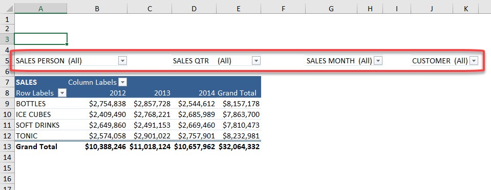
The layout of our filters has changed!

All the filters are now displayed in a horizontal format next to each other! If you want to change the layout back to vertical but this time you can limit the number of rows in the list.

Let’s see how it can be done!

 

Method 2: Limit Row in Vertical Format

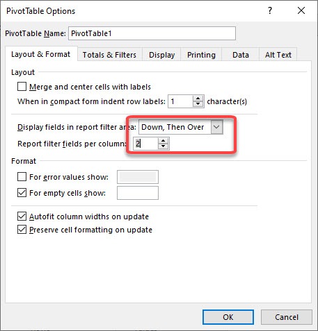
STEP 1: Let us try another setup. Go back to PivotTable Analyze > PivotTable > Options

STEP 2: Set it to Down, Then Over, and set the Report filter fields per column to 2.

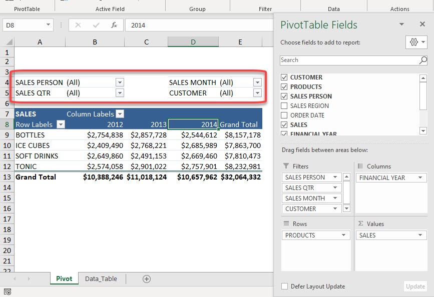
You now have a 2-column layout for your filters!

 

If you want a vertical arrangement, you can select Down, Then Over option

For a horizontal arrangement, you can select Over, Then Down option.

 

Click here to know Top 50 things that you can do with Excel Pivot Table!

 

Make sure to download our FREE PDF on the 333 Excel keyboard Shortcuts here: