Change Sum View in Label Areas

Exercise Workbook:

STEP 1: Here is our Pivot Table. Drag the Sales field to the Values area.

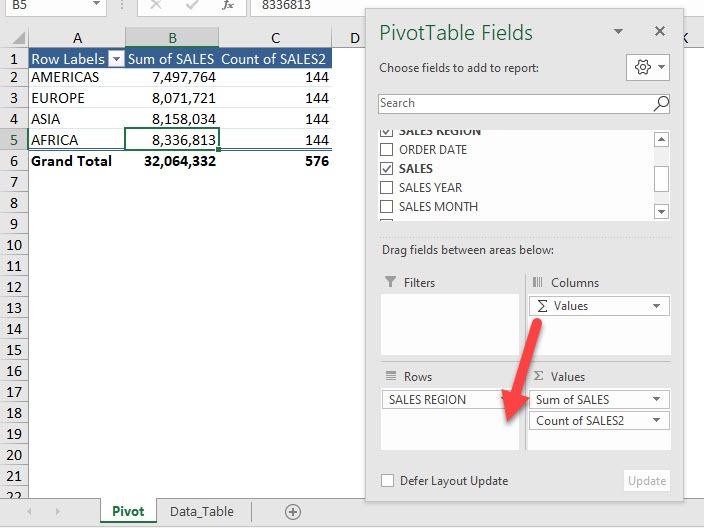
Notice we have the Sum of Values field added as well into the Columns area. This happens because we have more than one metric in our Values area.

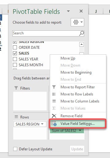
STEP 2: Let us change the second Sum of Sales field into Count. Click on the arrow and select Value Field Settings

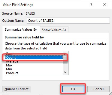
STEP 3: Select Count and click OK

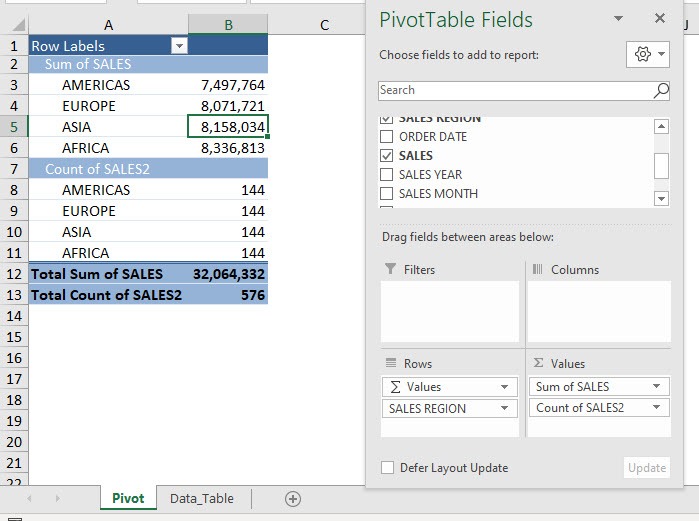
STEP 4: Now that we have our count, drag the Sum of Values field to the Rows area and see what happens!

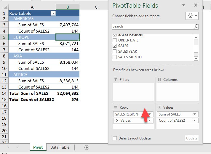
STEP 5: We have a completely different view. Now try moving the Sum of Values field above the SALES REGION field

And there you have the different views just by moving the Sum of Values field!

Make sure to download our FREE PDF on the 333 Excel keyboard Shortcuts here:

Bryan

Bryan Hong is an IT Software Developer for more than 10 years and has the following certifications: Microsoft Certified Professional Developer (MCPD): Web Developer, Microsoft Certified Technology Specialist (MCTS): Windows Applications, Microsoft Certified Systems Engineer (MCSE) and Microsoft Certified Systems Administrator (MCSA).

He is also an Amazon #1 bestselling author of 4 Microsoft Excel books and a teacher of Microsoft Excel & Office at the MyExecelOnline Academy Online Course.