Clean Data Set for Pivot Table

When working with Excel Pivot Tables, you will need to ensure that you have a clean data set. So there are 2 things that I want to show you:

• When your data is not clean
• How to clean your data.

Key Takeaways

• Ensure Column Headers Are Clear and Unique – Pivot Tables rely on distinct, non-blank headers in the first row of your dataset to function properly.

• Remove Blank Rows and Columns – Gaps in your data range can break Pivot Table references and lead to incomplete analysis.

• Convert to Excel Table Format – Use Ctrl + T to turn your data into an Excel Table for dynamic range updates and cleaner structure.

• Standardize Data Types – Make sure each column contains only one type of data (e.g., text, dates, numbers) for consistent aggregation and filtering.

• Check for and Remove Duplicates – Use Remove Duplicates or Power Query to avoid inflated counts or inaccurate summaries in your Pivot Table.

How to Clean Data Set for Pivot Table

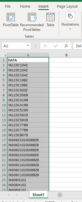
STEP 1: Here is our data set, select the data and go to Insert > Tables > PivotTable

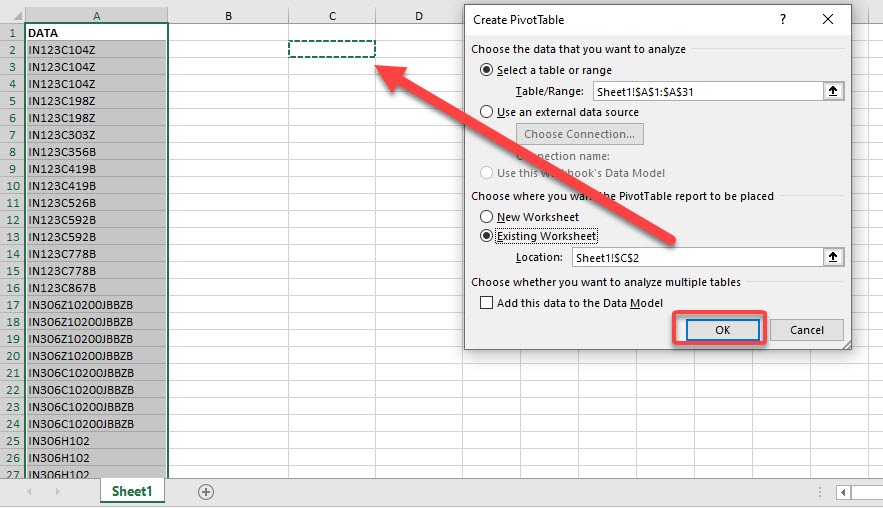
STEP 2: Select Existing Worksheet and pick a cell inside the same worksheet to insert our Pivot Table. Click OK.

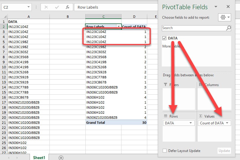
STEP 3: Drag the DATA column into Rows and Values

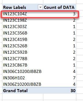
You will notice that how come IN123C104Z is appearing as 3 rows? This is caused by our dirty data!

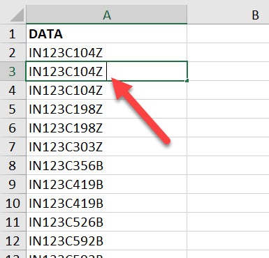
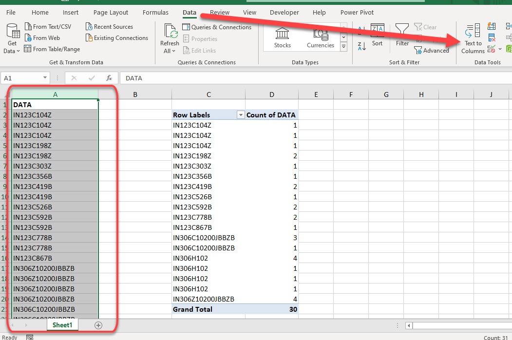
STEP 4: If you inspect the data table closely, you will see that they have extra spaces. This is what’s causing our Pivot Table to have weird outputs!

STEP 5: Let us clean those extra spaces! Select the entire column of your data and go to Data > Data Tools > Text to Columns

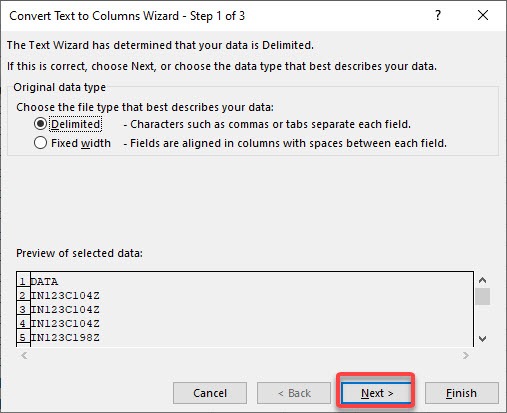
STEP 6: Click Next

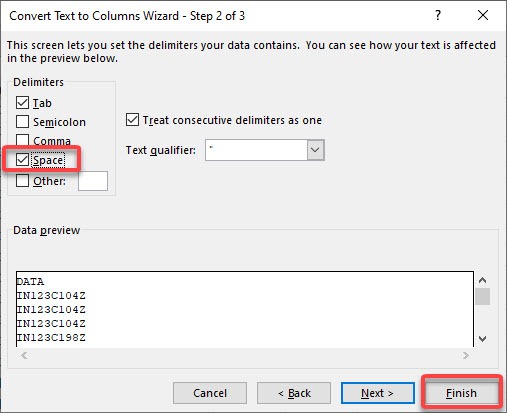
STEP 7: Make sure Space is ticked and select Finish. This will remove the extra spaces as a result.

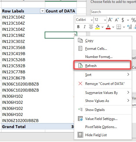
STEP 8: Right click anywhere on your Pivot Table and select Refresh to reflect our data cleanup.

Now that’s looking much better!

Frequently Asked Questions

Why is my Pivot Table not recognizing all my data?
Your dataset may contain blank rows or unrecognized formats that interrupt the data range. Ensure it’s continuous and formatted correctly.

What’s the benefit of converting data to an Excel Table?
Excel Tables auto-expand when you add data, making it easier to refresh Pivot Tables without redefining the range.

Do I need to sort the data before using it in a Pivot Table?
Not necessarily. Pivot Tables will sort data for you, but removing unnecessary sorting or formatting issues can help performance.

How can I find hidden issues in my data set?
Use Go To Special > Blanks or tools like Power Query to reveal hidden nulls, inconsistencies, or misaligned values.

What should I do if I see incorrect totals in my Pivot Table?
Check for text values in numeric columns or inconsistencies in data formatting that may prevent correct calculations.