Clear a #REF error in Excel

As someone who regularly uses Microsoft Excel, encountering a #REF! error can be both frustrating and confusing. I remember the first time I saw that glaring #REF! in one of my formulas—it felt like my entire spreadsheet was on the brink of collapse. Over time, I’ve learned not only why these errors occur, but also the best ways to tackle and prevent them. In this article, I’ll walk you through how I clear a #REF error in Excel, breaking down the process step by step so you can regain control of your data. I’ll cover common causes, troubleshooting techniques, preventative strategies, and more, all while sharing the tips that have saved me hours of headaches.

Key Takeaways:

• #REF! errors occur when a formula references cells, ranges, or sheets that no longer exist.
• I can often solve #REF! errors by undoing recent deletions or manually updating the formula to use valid references.
• Using named ranges and Excel Tables helps future-proof my formulas against accidental deletions or structural changes.
• Regularly backing up workbooks protects my data and formulas from irreversible errors.
• Tools like Trace Dependents/Precedents and Find and Replace streamline both troubleshooting and repairing #REF! errors, especially in large workbooks.

 

Understanding the #REF! Error

What is #REF! error in Excel?

From my experience, a #REF! error in Excel signifies that a formula is referencing a cell or range that no longer exists. Usually, this happens if I’ve deleted a row, column, or worksheet that the formula once pointed to. Excel uses #REF! as a placeholder to let me know that it can’t find the referenced data, and the formula can’t execute properly until it’s fixed.

Common Scenarios Leading to #REF! Errors

There are a few situations where I’m most likely to encounter this issue. The most common is deleting cells, rows, or columns that my formulas depend on. Another is copying or moving formulas to a different part of the worksheet, causing their references to shift to invalid locations. Sometimes, using cut and paste instead of copy and paste can also break references and trigger the dreaded #REF! error.

 

How to fix #REF error in Excel?

Example 1: Fixing #REF! Error Caused by Deleted Cells in a Formula

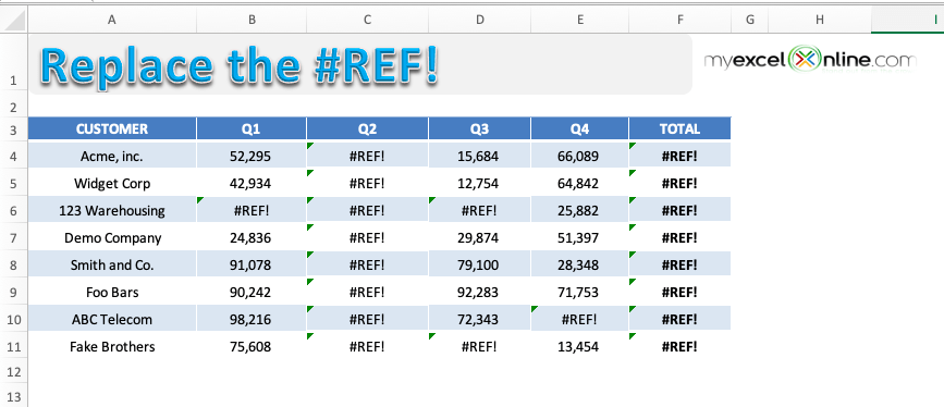
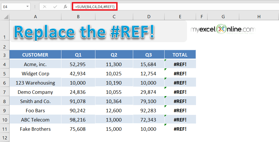
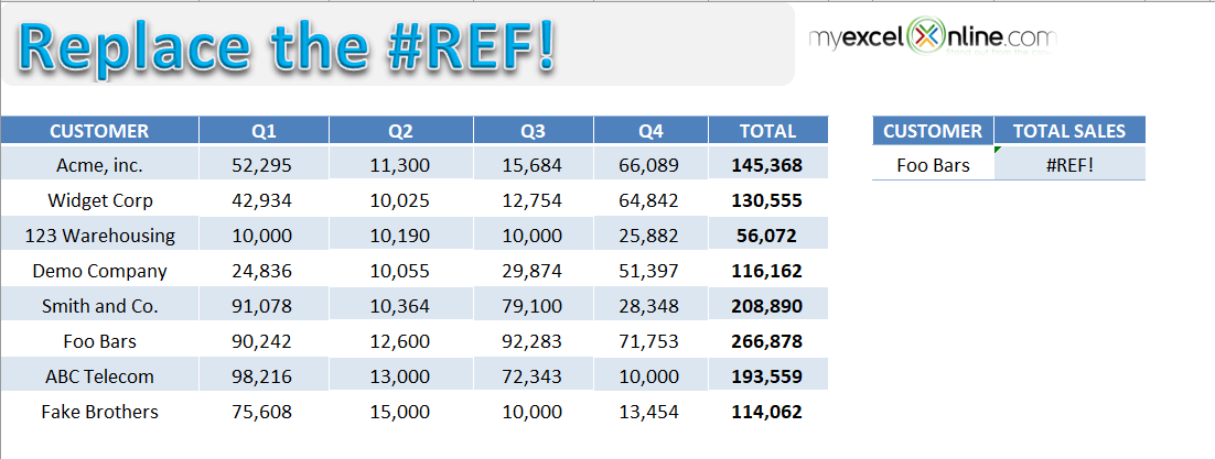
In the table below, you will spot multiple #REF! error within formulas used in the cell.

This has happened because you have deleted a range that contains an explicit cell reference within the formula used.

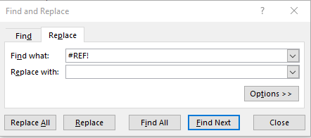
To get rid of this error message we have to select the cell(s) with this error, use the Find & Replace dialog box and do the following:

Find What: #REF!

Replace With:   (Leave this blank)

Press OK and it will clear the #REF error in Excel within the formula.

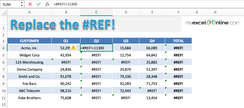
STEP 1: To check the cell containing the cell, simply click on the cell and press F2.

Here, since you have used an explicit cell reference and it was deleted, Excel is returning a #REF error.

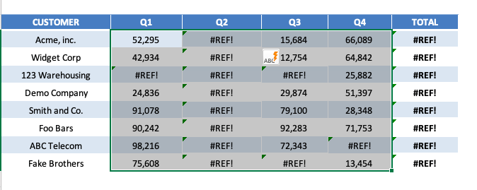
STEP 2: Highlight the table containing the errors.

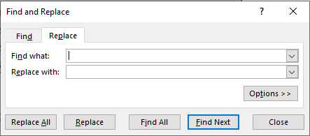
STEP 3: Press Ctrl + H to open the Find & Replace dialog box.

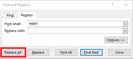
STEP 4: Under Find What, input #REF! and leave Replace as blank. This is done to replace all the #REF! error with a blank.

STEP 5: Click on Replace All.

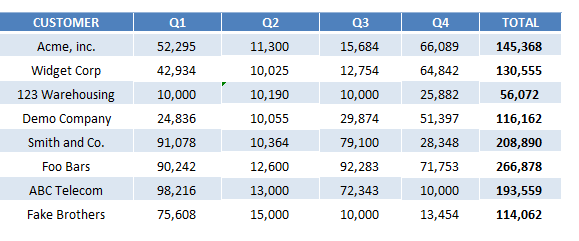
This is how your replaced data will look like:

Let’s look at another example when this error occurs due to copy-pasting the formula from other cells.

Example 2: Avoiding #REF! Error When Deleting Columns with SUM Formula

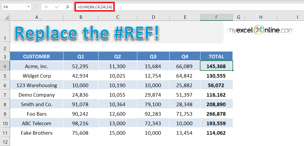
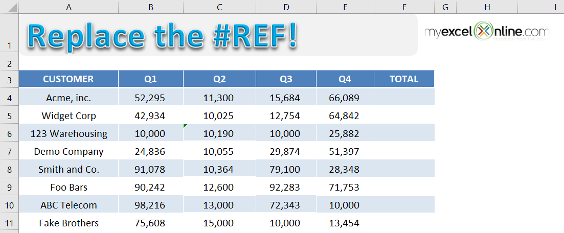
In the table below, you have sales data for different customers for 4 quarters and a sum formula used to calculate the total sales. The formula used to calculate the total sales value is =SUM(B4, C4, D4, E4).

If you try and delete Column E (Quarter 4), the sum formula will change to =SUM(B4, C4, D4,#REF!) and return an error – #REF.

This error is caused because the formula to calculate the total sales uses explicit cell reference. When one of the cell references used in the formula is deleted (here cell E4), Excel is unable to calculate the value and returns an error.

A simple fix to this problem is to use a range instead of an explicit cell reference. Let’s look at the step-by-step tutorial to learn how:

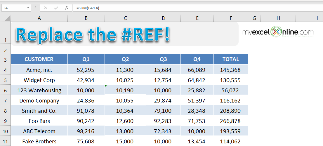
STEP 1: Use formula =SUM(B4: E4) in cell F4 and copy-paste the formula below to cells F5: F11.

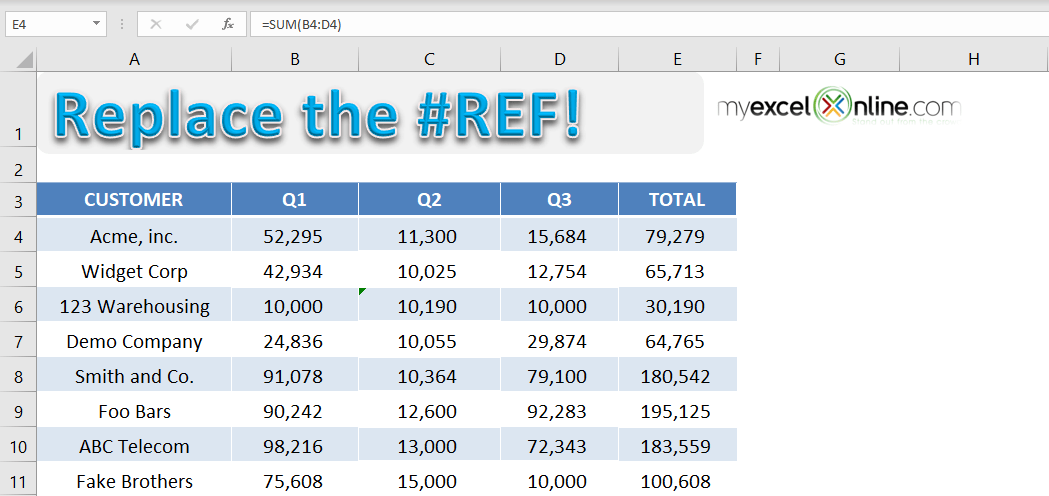
STEP 2: Now delete the Column E to get the total sales for only 3 quarters.

If you change the formula from =SUM(B4, C4, D4, E4) to =SUM(B4: E4), you will no longer to vulnerable to #REF in Excel. This formula recalculates the total sales value by removing the deleted cell.

Hence, it is advised to use range while writing a formula instead of explicit cell reference.

Let’s take a look at another example when the error occurred due to VLOOKUP containing invalid cell reference.

Example 3: Resolving #REF! Error in VLOOKUP Due to Invalid Column Index

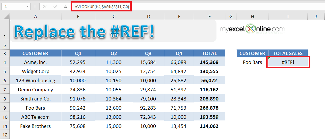
In the table below you have quarterly and total sales for different customers and using the VLOOKUP formula, you have tried to find out the total sales for the customer name mentioned.

The formula used to find the total sales for customers mentioned in cell H4 is =VLOOKUP(H4,$A$4:$F$11,7,0).

If you look into the formula used in detail, you will see that the value used to indicate the column index number is incorrect.

The arguments for a VLOOKUP function is:

• Lookup_value = The value you want to look up in the first column of the table.
• Table_array = The table from which you need to retrieve the data.
• Col_index_num = The column number in the table array from which matching value should be returned.
• Range_lookup = Value should be 1 if you want an approximate match or 0 if you want an exact match of the return value.

Excel is returning an error in this formula because VLOOKUP is looking to return a value from the 7th column but the reference $A$4:$F$11 contains only 6 columns.

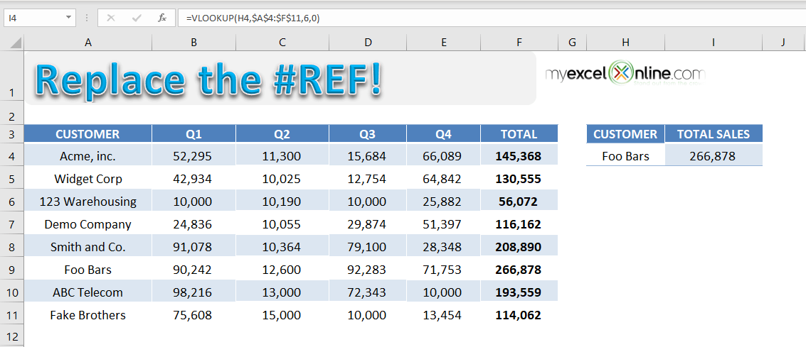
To fix this error, use the formula =VLOOKUP(H4,$A$4:$F$11,6,0).

 

FAQs

1. What is #REF! error in Excel?

The #REF! error in Excel means that a formula is referring to a cell, range, or sheet that no longer exists. This usually happens when a referenced cell gets deleted or when the structure of your workbook changes in a way that breaks the link. It’s Excel’s way of saying, “I’m lost—where do you want me to look?” Until the formula is corrected, Excel can’t calculate anything based on that broken reference.

2. How do I identify which cell or formula is causing the #REF! error?

To pinpoint the cause, click on the cell with the error and press F2 to enter edit mode. This will highlight the formula and show you exactly where the #REF! is appearing. Excel also gives you a tooltip when you hover over the error, offering hints about what went wrong. If you’re dealing with a large sheet, use the Find (Ctrl+F) function to search for all occurrences of #REF!.

3. Can I use Find & Replace to fix all #REF! errors at once?

Yes, you can use Ctrl + H to open the Find & Replace dialog and search for #REF!. Leave the “Replace with” field blank and click Replace All to quickly clean up your sheet. However, this only removes the error—it doesn’t restore the original references. So while it’s useful for bulk cleanup, it’s not a true fix unless you’re okay with leaving those cells empty or handling them manually afterward.

4. Why do #REF! errors often appear after deleting columns or rows?

When you use explicit references like =SUM(B4, C4, D4, E4), deleting any of those columns will cause Excel to lose track of the reference and throw a #REF! error. This is because the formula doesn’t automatically adjust when a referenced cell is removed. To prevent this, use range references like =SUM(B4:E4)—they adapt better to structural changes and reduce the risk of errors.

5. How can I avoid #REF! errors when using formulas like VLOOKUP?

#REF! errors in VLOOKUP typically occur when the column index number is greater than the number of columns in your table array. For example, if your range is $A$4:$F$11, then your column index must be 1 to 6—not 7. Always double-check the size of your lookup range and ensure your column index stays within that boundary. Alternatively, consider using INDEX/MATCH for more flexibility and fewer errors.