How to Convert Column Numbers to Letters in Excel

Unlocking the secrets behind Microsoft Excel‘s column identifiers can greatly enhance your efficiency. Understanding the logic of Excel’s column lettering system and learning to convert between column letters and numbers will make navigating your spreadsheets easier. This guide covers essential techniques, including the CHAR and ADDRESS functions, and practical VBA code snippets for automation.

Key Takeaways:

• Understanding Excel Column Identifiers: Excel’s column system repeats letters after ‘Z’ (e.g., ‘AA’, ‘AB’), simplifying navigation and referencing.
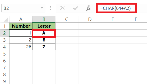
• Using the CHAR Function: The CHAR function converts column numbers to letters using ASCII codes (e.g., =CHAR(64 + column_number)).
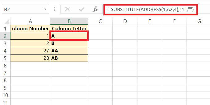
• ADDRESS Function for Dynamic References: Combined with SUBSTITUTE, the ADDRESS function dynamically converts column numbers to letters (e.g., =SUBSTITUTE(ADDRESS(1, column_number, 4), “1”, “”)).
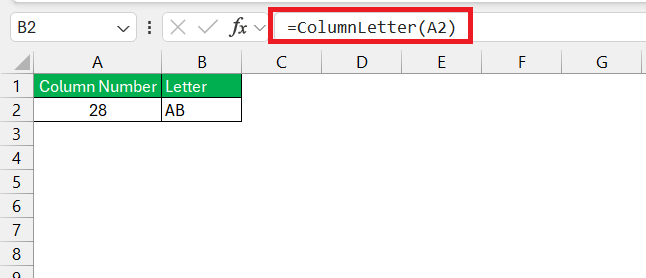
• Automating with VBA: VBA code snippets can automate column number-to-letter conversions, enhancing productivity (e.g., Public Function ColumnLetter(col_num As Integer) As String).

 

Unlocking the Secrets of Excel Columns

The Mystery Behind Column Identifiers

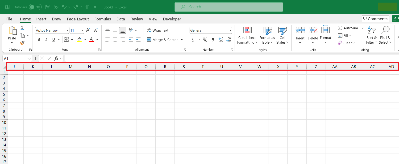
Excel’s column identifiers might seem cryptic at first glance, but they actually follow a simple pattern. It’s similar to the alphabet, where after ‘Z’, the letters repeat with ‘AA’, ‘AB’, and so forth. Understanding this can transform the way you navigate and use Excel.

 

The Fast Track to Excel Mastery

When Numbers Become Letters

Excel typically uses letters for column headings, which can be pretty handy, but sometimes you’ll need to convert these to their corresponding numerical position. This is particularly true when dealing with Excel functions or programming within Excel. They must translate that ‘A’ into ‘1’, ‘B’ into ‘2’, and it gets a bit trickier once you pass ‘Z’. But don’t worry, you’ll soon have the tips to make that conversion a breeze.

In Excel, the CHAR function returns the character specified by a number (character code) from the character set used by your computer. The CHAR function returns a character based on its ASCII code. The ASCII values for uppercase English letters range from 65 (A) to 90 (Z).

Therefore, to find the ASCII code for an uppercase letter, you add its position in the alphabet to 64. For instance, for ‘A’ (the 1st letter), you add 1 to 64 to get 65; for ‘B’ (the 2nd letter), you add 2 to 64 to get 66, and so on.

Note: If dealing with columns beyond ‘Z’ (i.e., past 26), you’ll need a different approach, as Excel column letters repeat after ‘Z’. In such cases, use a combination of the ADDRESS and SUBSTITUTE functions.

Your Toolkit for Column Conversion

The Indispensable ADDRESS Function

The ADDRESS function is a game-changer for when you need to convert row and column numbers into a cell address. It’s the perfect tool to construct dynamic cell references, and when you’re manipulating data programmatically. With it, you can say goodbye to manually inputting cell addresses and hello to efficiency. For instance, if you’re dealing with the column number, simply set the row number to 1 and the reference style to 4 (for relative referencing) to get just the column letter.

To convert column numbers to letters using the ADDRESS function, follow this step:

Use the formula =SUBSTITUTE(ADDRESS(1,A2,4),”1″,””). The 1 sets the row, and 4 ensures relative referencing.

This efficiently generates the column letters.

 

Nifty Tricks for Power Users

Creating Custom Functions for Lightning-Fast Results

For those of you who love to work smarter, not harder, creating custom functions in Excel is the way to go. Excel’s built-in functions are powerful, but sometimes, they don’t fit the specific need you have. By writing your own function, say to convert column numbers to letters, you can save heaps of time with a formula that does exactly what you need with a single call. Get ready to impress with your newfound speed!

Automating Conversion with VBA Code Snippets

Dive into the world of automation with VBA code snippets and watch your productivity soar. By using the Visual Basic for Applications editor in Excel, you can write a snippet of code that turns tedious column number-to-letter conversions into a one-click affair. Whether it’s a one-time project or a regular necessity, these snippets can be your time-saving secret weapon. Just remember to save your code after creation for reuse in future projects.

The following code can be used as VBA:

Public Function ColumnLetter(col_num As Integer) As String

ColumnLetter = Split(Cells(1, col_num).Address, "$")(1)

End Function

 

Practical Applications and Use Cases

Organizing Data Like a Pro

To organize your data like a seasoned Excel pro, consider using named ranges — you can refer to cells by names, making your formulas easier to read and manage. Utilize the ‘Sort & Filter’ feature to rearrange your data in meaningful ways, whether alphabetically or based on numerical values. Don’t forget to group rows or columns to declutter your view. Mastering these organizational tactics ensures your data is always presented cleanly and logically.

Enhancing Readability and Navigation

Enhancing the readability and navigation of your Excel spreadsheets invites clarity and efficiency into your work. Consider applying conditional formatting to highlight key data, freeze panes to keep header rows and columns in view as you scroll, and use data validation to make sure the inputs are within a desired range. To further improve navigation, implement drop-down lists and create interactive buttons or links to jump to different sections. These strategies make large data sets more approachable and user-friendly.

FAQs: Quick Solutions to Common Queries

How to convert Excel column number to letter?

To convert an Excel column number to a letter, you can use the ADDRESS function together with SUBSTITUTE:

=SUBSTITUTE(ADDRESS(1, your_column_number, 4), "1", "")

Replace your_column_number with the actual column number you’re converting. This formula will give you the column letter as a result.

How can I convert a column number to a letter in Excel directly?

For a direct conversion of a column number to a letter in Excel, utilize:

=CHAR(64 + your_column_number)

If dealing with columns beyond ‘Z’ (i.e., past 26), you’ll need a different approach, as Excel column letters repeat after ‘Z’. In such cases, use a combination of the ADDRESS and SUBSTITUTE functions.

How do I change the column headings back to letters such as a, b, c, d?

To change column headings back to letters in Excel, go to the ‘File’ tab, click ‘Options’, then ‘Formulas’, and uncheck the ‘R1C1 reference style’. Click ‘OK’ and your column headings will switch back to the alphabetical system.

Is there a way to toggle between letter and number column headings?

Yes, you can toggle between letter and number column headings in Excel. Go to ‘File’ > ‘Options’ > ‘Formulas’, and check or uncheck the ‘R1C1 reference style’ box to switch between the two systems. Remember to click ‘OK’ to apply the changes.

How can we get the column letter for the given specific cell in microsoft excel?

To get the column letter for a specific cell in Excel, use the following formula:

=SUBSTITUTE(ADDRESS(1, COLUMN(your_cell_reference), 4), "1", "")

Replace your_cell_reference with the cell you’re interested in, like A1 or B2, and the result will be the column letter of that cell.