The Basics:
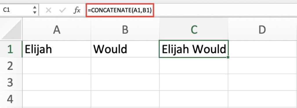
In Excel, the CONCATENATE function basically combines 2 or more cells of strings. In our previous blog entitled Concatenate in Excel – With and Without a Separator, we learned how to combine 2 cells into 1, as shown:
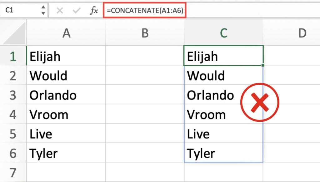
Although you can input the references individually within the CONCATENATE function, it would not function properly if you input a range of cells as a reference.
As you can see, the formula above does not combine the range of cells into one cell.
In this article, we will explore CONCATENATE Excel Range with and without separators, offering you a comprehensive guide to mastering this essential Excel function.
Let’s explore these methods!
Download the Excel Workbook below to follow along and understand How to Combine Cell Ranges in Excel – download excel workbookConcatenate-Range.xlsx
Click here to access Microsoft’s tutorial on the CONCAT Function!
Concatenate Excel Range Without Separator
Let’s start with the basics: combining data without any separator. This is super handy when you want to combine text from different cells into a single cell, maintaining the original formatting. Follow these steps:
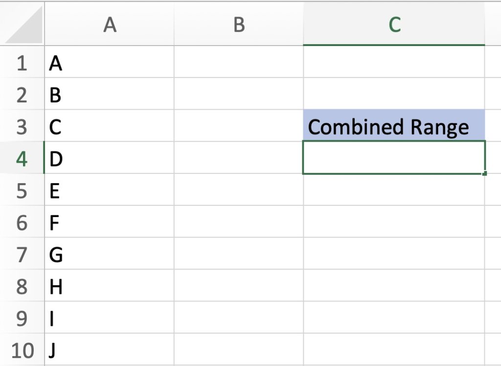
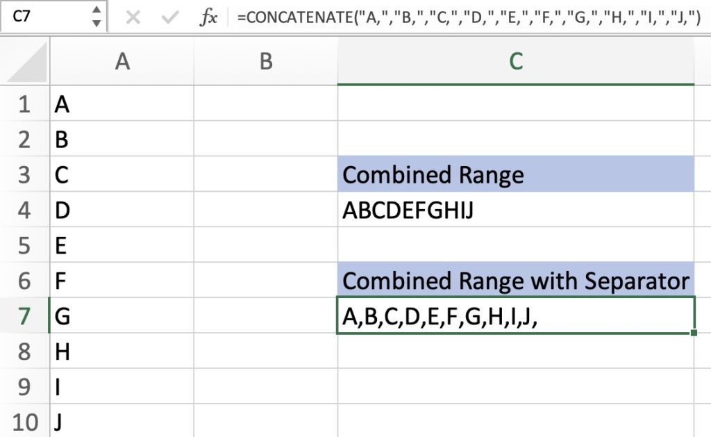
Select the cell where you want the merged data. In our case, it is C4.
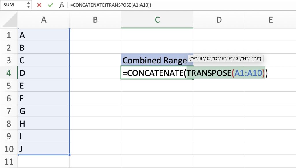
In the formula bar, enter =CONCATENATE(TRANSPOSE(A1:A10))
Highlight TRANSPOSE(A1:A10) from the formula and press F9. (Or use Fn+F9 on a Mac) This converts that part of the formula into values.
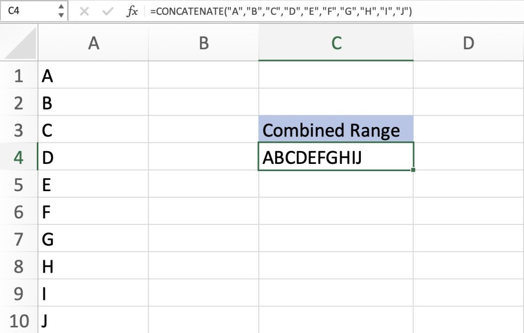
Remove the middle brackets at both ends.
Press Enter.
There you have it! We’ve successfully merged the range of cells into one cell without any separator.
Concatenate Excel Range With Separator
Now, let’s learn how to concatenate an Excel range with a separator. In this scenario, we will add a specific character or symbol between the combined values, such as a space, comma, or hyphen. Follow these steps to do it:
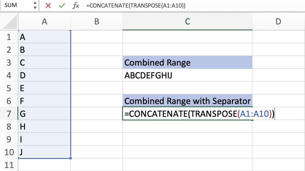
Select the cell where you want the merged data. In our case, it is C7.
In the formula bar, enter =CONCATENATE(TRANSPOSE(A1:A10))
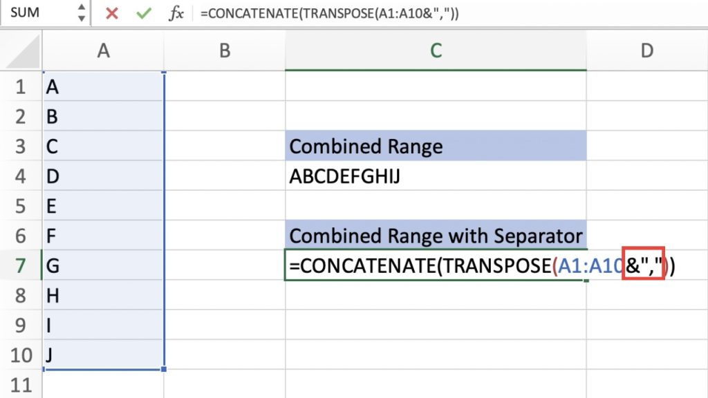
Now, for the magical part: After the range, input the ampersand sign (&) and whatever separator you want to use in between quote signs (“”). In our case, we will use a comma.
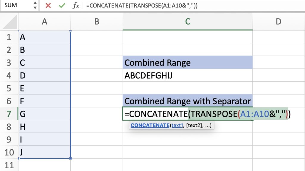
The formula will now be =CONCATENATE(TRANSPOSE(A1:A10&”,”))
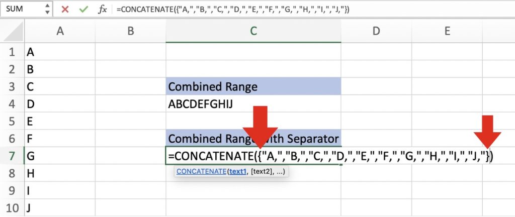
Highlight TRANSPOSE(A1:A10&”,”) from the formula and press F9 (Or use Fn+F9 on a Mac) to convert that part of the formula into values.
Remove the middle brackets at both ends.
As you can see, we’ve successfully combined the range of cells into one cell, this time with a space character as the separator. You can easily replace the space with any other character, such as a comma or hyphen, to accommodate your needs.
Hopefully, this will help you cut down on the time and energy needed to handle big sets of data. Once you’ve got the hang of using CONCATENATE in Excel, whether with or without spacing in between, you’ll find yourself breezing through your spreadsheet work.
Further learning:
- Concatenate in Excel – With and Without Separator
- CONCAT Formula in Excel
- 3 Easy ways to Concatenate Excel With A Line Break
Click here to learn more about the CONCATENATE function in Excel!
John Michaloudis is a former accountant and finance analyst at General Electric, a Microsoft MVP since 2020, an Amazon #1 bestselling author of 4 Microsoft Excel books and teacher of Microsoft Excel & Office over at his flagship MyExcelOnline Academy Online Course.

