How to Compare Text in Cells for Precision Work in Excel

Comparing text in Excel can seem like a daunting task at first, but trust me, it’s easier than you might think. Whether you’re working on cleaning up data, identifying duplicates, or checking for specific keywords, Excel provides a range of tools and formulas that make text comparison a breeze. Let me walk you through the different methods I use to compare text in Excel effectively.

Key Takeaways:

• Excel offers versatile tools for text comparison, from simple formulas to advanced Power Query techniques.
• The EXACT function is ideal for case-sensitive text comparisons, ensuring precise results.
• Conditional formatting visually highlights differences, simplifying data review.
• Functions like SEARCH and FIND are excellent for partial matches, with options for case sensitivity.
• Power Query provides a robust solution for comparing large datasets or performing complex analyses.

 

Unlocking the Secrets of Text Comparison in Excel

The Art of Zeroing in on Text Differences with Excel Tools

Comparing text in Excel might seem daunting, but upon closer examination, I’ve found an array of tools within Excel that can simplify this task for us. Although Excel was not traditionally known for its text comparison capabilities, the situation has been changing with third-party add-ins and some ingenious techniques that we can use to find text differences efficiently.

Enhancing Precision in Data Analysis: A Closer Look at Text Comparison

Text comparison is integral to enhancing precision in data analysis, ensuring accuracy down to the smallest detail. When I delve into datasets that contain textual elements, the accuracy of my results often hinges on how well I can discern even the most minute discrepancies. Excel offers functionalities that make it possible to compare text, identify, and even highlight these differences, which is pivotal in tasks such as reconciling accounts, deduplicating data, or integrating datasets from varied sources.

By incorporating rigorous methods of text comparison, we can substantially reduce the margin of error and bolster the integrity of our analyses. Leveraging Excel’s tools, I find that I can transform a monotonous manual task into an automated, reliable process.

 

Step-by-Step Guide to Master Compare Text

Method 1: Using the EXACT Function

The EXACT function is my go-to tool when I need to check if two text strings are identical, including their case sensitivity.

Here’s how I use it:

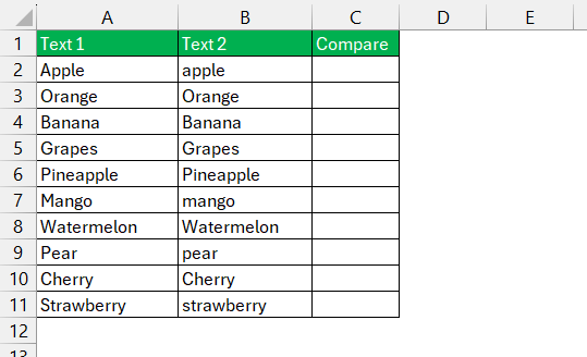
STEP 1: Suppose I have two columns, A and B, with text values. I want to compare text in these columns row by row.

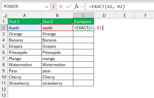
STEP 2: In column C, I enter the formula:

=EXACT(A2, B2)

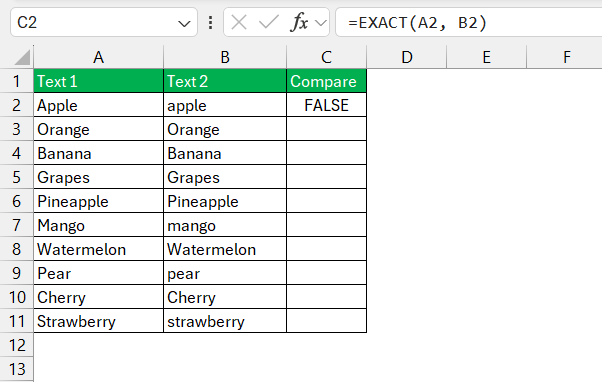
STEP 3: After pressing Enter, Excel will return TRUE if the two text strings are an exact match and FALSE if they are not.

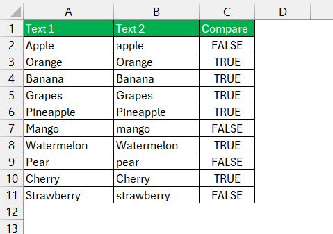
STEP 4: I can then drag this formula down the column to compare the rest of the rows.

This method is super useful when I’m working with case-sensitive data, like passwords or specific codes.

Method 2: Using the Equal Sign (Case Insensitive)

If case sensitivity isn’t a concern, I often use a simple formula to compare text:

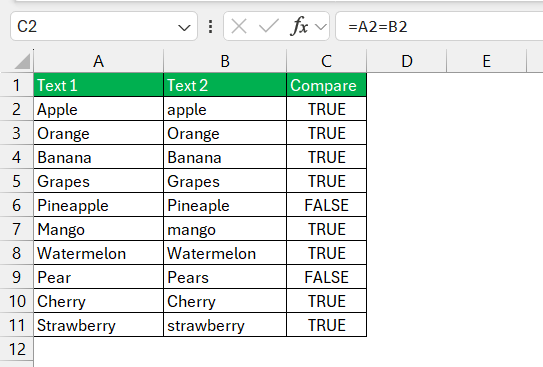
Again, with two columns of text, I enter the following in column C:

=A2=B2

This will return TRUE if the values are the same (ignoring case) and FALSE otherwise. It’s quick, easy, and works perfectly for most scenarios.

Method 3: Highlighting Differences with Conditional Formatting

Sometimes, I need to visually spot differences between two columns of text. Conditional formatting is a lifesaver for this.

Here’s what I do:

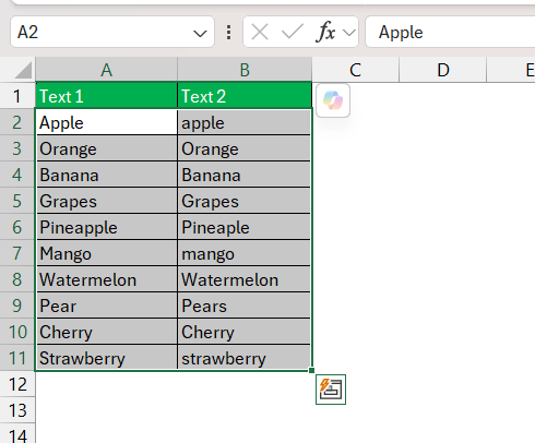
STEP 1: I select the range of cells I want to compare (e.g., A2:A11 and B2:B11).

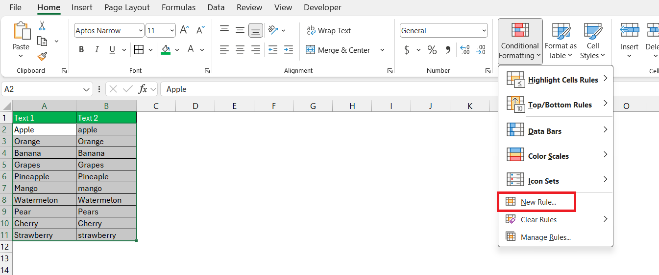
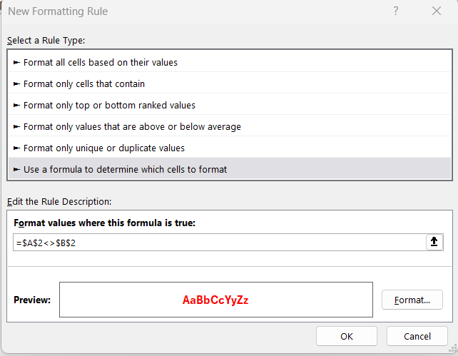
STEP 2: I go to the Home tab, then click on Conditional Formatting > New Rule.

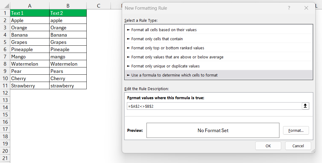
STEP 3: I choose “Use a formula to determine which cells to format” and enter this formula:

=A2<>B2

STEP 4: I set a formatting style, like a bold red fill, to highlight cells where the text doesn’t match.

After clicking OK, Excel instantly highlights the differences, making them easy to spot.

Method 4: Checking for Partial Matches

When I’m searching for specific keywords or checking if one text contains another, I use the SEARCH or FIND function.

Here’s an example:

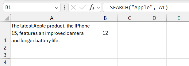
If I want to check if the text in column A contains the word “Apple”, I use:

=SEARCH(“Apple”, A1)

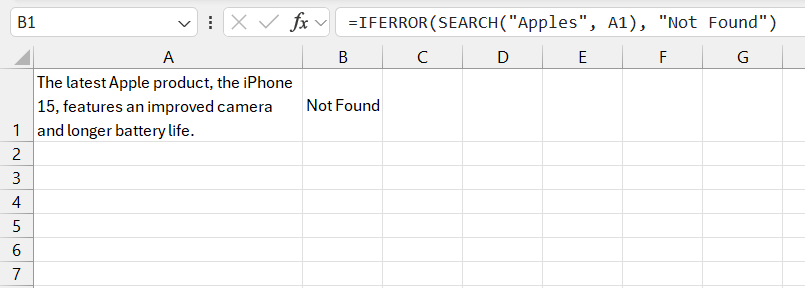
This returns the position of the word “Apple” in the text, or an error if it’s not found. To avoid errors, I often wrap it in an IFERROR function:

=IFERROR(SEARCH(“Apples”, A1), “Not Found”)

The SEARCH function is case-insensitive, but if I need case sensitivity, I switch to FIND.

 

FAQ

How do you compare text in Excel?

To compare text in Excel with case sensitivity, the EXACT function is your best option. This function compares two text strings exactly, including any differences in upper or lowercase letters. It returns TRUE if the strings are identical, considering case, and FALSE if there are any discrepancies. This is particularly useful for sensitive data, such as passwords or specific codes, where case differences matter.

What are the Go-to Functions for Precise Text Comparisons?

For case-insensitive text comparison, use the formula =A1=B1. This simple formula checks whether the text in two cells is the same, ignoring any differences in letter case. If the two strings match, it will return TRUE; otherwise, it will return FALSE. This method is effective when the case of letters isn’t important, such as when comparing names or product descriptions.

Can I Compare More Than Two Columns for Text Differences in Excel?

To visually highlight differences between two columns, you can use conditional formatting in Excel. First, select the range of cells you want to compare and go to Home > Conditional Formatting > New Rule. Choose “Use a formula to determine which cells to format” and enter a formula like =A1<>B1, then apply a formatting style, such as a bold red fill. This method makes it easy to spot mismatches at a glance.

Are There Ways to Automate Text Comparison for Large Datasets?

For partial text matching, the SEARCH or FIND functions are highly effective. The SEARCH function allows you to locate a specific substring within a text string and is case-insensitive, while the FIND function is case-sensitive. You can use these functions to check if a certain word or pattern appears in a cell and return the position of the match. If no match is found, you can use IFERROR to return a custom message, such as “Not Found.”

Why is it useful to compare two columns in Excel?

Yes, you can compare entire datasets for mismatches using a helper column with a formula. A common approach is to use =IF(A1<>B1, "Mismatch", "Match"), which will flag rows as “Mismatch” or “Match” based on the comparison of corresponding cells in two columns. This method allows you to quickly identify differences between large datasets, ensuring that no discrepancies go unnoticed.