Compare Two Columns in Excel for Matches & Differences: 3 Useful Methods

Comparing two columns in Microsoft Excel can be essential for identifying matches or differences between datasets. Utilizing functions like VLOOKUP and MATCH, alongside Excel’s conditional formatting, provides multiple efficient approaches to pinpoint discrepancies and align data. These powerful tools allow users to conduct a thorough comparison, whether for reconciling records or analyzing information across columns.

Key Takeaways

• Utilize the VLOOKUP function to compare two columns by searching a value from one column in another and returning related content.
• Employ the MATCH function in Excel to locate the position of a specific item in a column, useful for comparing lists to see if a value exists.
• Create a conditional formatting rule to visually highlight matches or differences when comparing two columns, streamlining the identification process.
• To ensure accurate comparisons, avoid common pitfalls like mismatched data types, leading/trailing spaces, and formula errors.

 

Unlocking Excel’s Potential

The Power of Data Comparison in Excel

Excel’s capability to compare data across columns is a game-changer for anyone looking to conduct thorough data analysis. This function is integral in data-driven environments, allowing for meticulous examination of inconsistencies, identification of unique values, and assessment of data trends. Proper data comparison can unlock insights that could be critical for decision-making and performance improvement. By knowing how to wield this tool, one can ensure data integrity and gain a competitive edge in data management.

 

Getting Started with Column Comparison

Preparing Your Spreadsheet for Match Hunting

When embarking on a journey to find matches across columns, the initial step involves preparing your spreadsheet. This preparation includes cleaning your data, removing duplicates, and ensuring that the data formats are consistent across both columns. Key preparation measures include:

• Standardizing Data Formats: Before comparing, make sure that the data formats match, particularly in the case of dates, currencies, and other numerical data, to prevent erroneous mismatches.
• Sorting and Filtering: Sort your data to align similar values and use filters to weed out unnecessary information, focusing on the area of comparison.
• No More Blank Spaces: Empty cells can be misleading during the comparison process. Fill or remove blank cells to maintain accuracy in your results.
• Identify Headers: Mark headers for each column. Descriptive and distinct headers facilitate easier navigation and understanding of the data you are matching.

By meticulously preparing your data, you set the stage for a refined and efficient matching process. This paves the way for the application of basic or advanced data comparison techniques in Excel

 

Advanced Strategies for Excel Wizards

Taking VLOOKUP Beyond the Basics

VLOOKUP is a staple in Excel for comparing two columns, but there are ways to enhance its functionality for more complex tasks. The VLOOKUP function can be used to search for a value in the first column of a range or table, and then return a value in the same row from a specified column. To compare two columns:

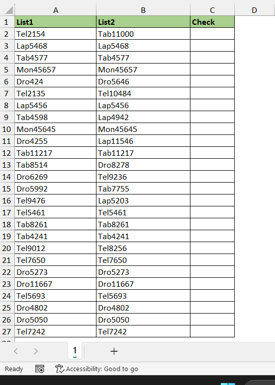
STEP 1: Prepare your data. Ensure Column A contains the values you want to search for, and Column B contains the values you want to search within.

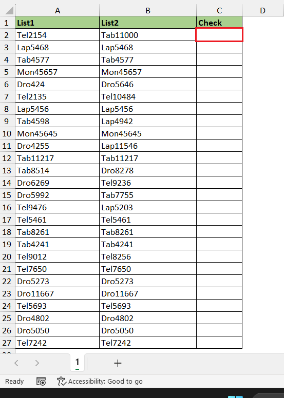
STEP 2: Select the cell where you want to display the first comparison result: This should be the first cell in Column C next to your first value in Column A (e.g., C2).

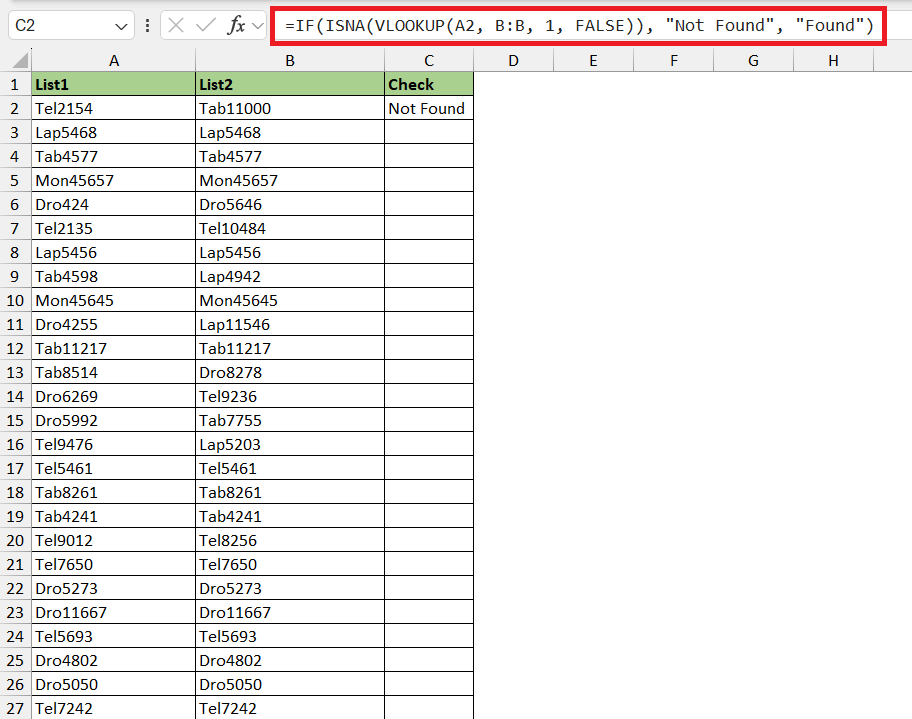
STEP 3: Enter the VLOOKUP formula: Type the following formula into the selected cell:

=IF(ISNA(VLOOKUP(A2, B:B, 1, FALSE)), “Not Found”, “Found”)

Here, A2 is the first value you’re searching for. B:B indicates the column range where you’re searching. 1 means you’re retrieving the first column’s value in the lookup range, which is necessary for the VLOOKUP function to work, even though we only use it to check existence. FALSE specifies an exact match.

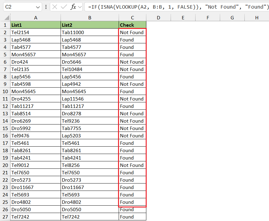
STEP 4: Copy the formula down the column: Drag the fill handle (a small square at the bottom right corner of the cell) down to copy the formula for all other values in Column B.

By mastering this VLOOKUP technique, you’ll be able to tackle more intricate data analysis tasks and enhance the efficiency and accuracy of your work in Excel.

 

The Sleight-of-Hand With MATCH

While VLOOKUP has its merits, the MATCH performs a nimble sleight-of-hand that brings unmatched flexibility to data comparison in Excel. Here’s how you can compare two columns with esteeming finesse:

STEP 1: Prepare your data Columns A and B should be set up with the values to compare, as with the VLOOKUP method.

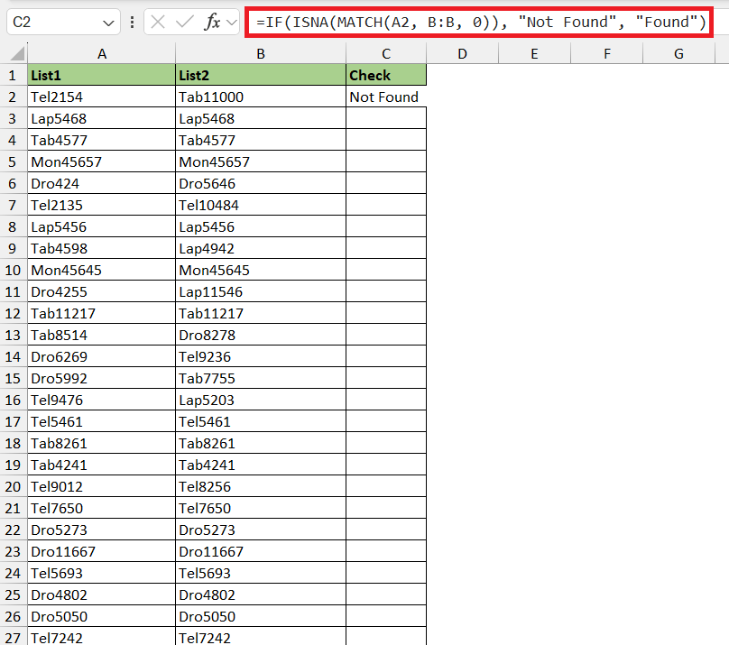
STEP 2: Select the cell for the first comparison result: This would typically be in Column C, starting with C2 adjacent to the first value in Column A. Enter the MATCH formula: Type the following formula into the cell:

=IF(ISNA(MATCH(A2, B:B, 0)), “Not Found”, “Found”)

A2 is the value you’re searching for. B:B is the range to search within. 0 indicates you’re looking for an exact match.

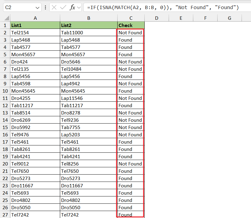
STEP 3: Copy the formula down the column: Drag the fill handle to apply the formula to the rest of the values in Column B.

By adopting the potent MATCH function, you unlock a higher level of productive data analysis, crafting comparisons that are resilient to changes and versatile in application. This method is lauded by Excel wizards for its proficiency in matching data and catering to a more nuanced data search and retrieval process.

 

Visual Tricks to Illuminate Matches and Differences

Conditional Formatting: A Rainbow of Possibilities

In a spreadsheet teeming with data, conditional formatting wields like a painter’s brush, adding vibrant hues to illuminate matches and distinctions between two columns:

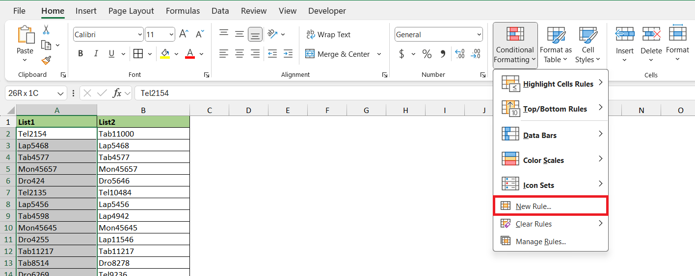
STEP 1: Select the range in Column A that you want to compare against Column B. This could be, for example, A2:A27.

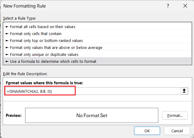
STEP 2: Go to the Home tab on the ribbon, click on “Conditional Formatting,” and then select “New Rule.”

STEP 3: Create a new rule based on a formula: Choose “Use a formula to determine which cells to format.” Enter the conditional formatting formula for comparison: Type in:

=ISNA(MATCH(A2, B:B, 0))

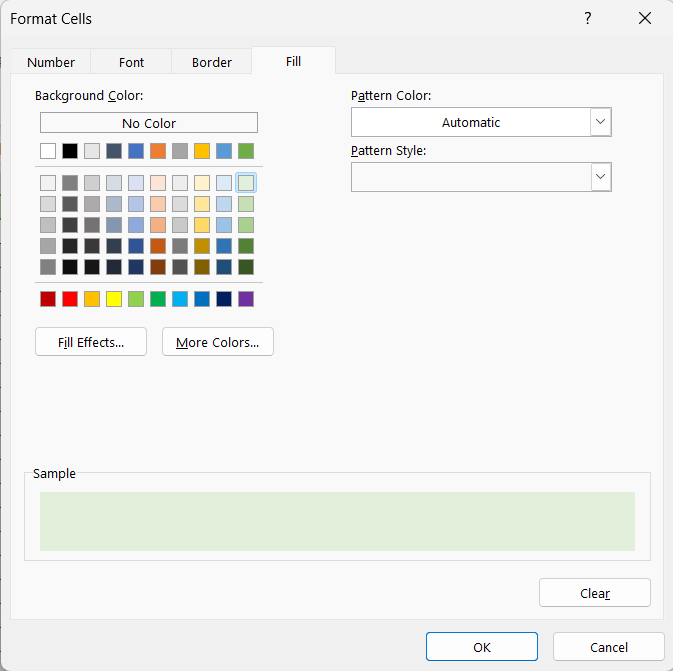
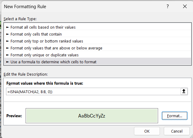
STEP 4: Click on the “Format” button, choose a fill color or text color to highlight cells, and then click OK to apply your formatting.

STEP 5: Finalize the rule. Click OK in the New Formatting Rule dialog to apply your conditional formatting.

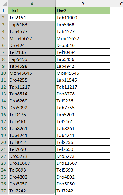
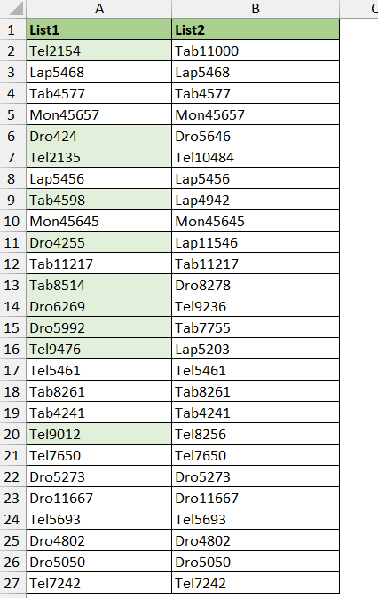
The result looks like this –

Utilizing these techniques, conditional formatting becomes a powerful ally in your Excel toolkit, capable of transforming columns of data into a vibrant, easily interpretable canvas. Whether you seek to quickly pinpoint data anomalies or bring harmony to matching values, conditional formatting offers a spectrum of possibilities to achieve your analytical goals with visual panache.

 

Best Practices for Spellbinding Results

Avoiding Common Pitfalls in Data Matching

Ensuring accuracy when matching data in Excel requires vigilance against common pitfalls that can lead to misleading analysis or flawed results. Here are the frequent missteps to avoid:

• Mismatched Data Types: Always check that the data types in the columns you’re comparing match. Numbers stored as text, or vice versa, will not equate and can be the root cause of unexpected mismatches.
• Ignoring Leading and Trailing Spaces: Invisible spaces before or after data entries can cause correct matches to fail. Utilize the TRIM() function to clean your data before analysis.
• Case Sensitivity Oversights: While Excel’s standard comparison functions are not case-sensitive, sometimes specific datasets require case-sensitive comparisons. Use the EXACT() function if the case is a significant factor in your comparison.
• Incorrect Range References: Dynamic data may extend past the original range set for comparison. Always verify that your formulas encompass the entire dataset, particularly when new data is added.
• Overlooking Hidden Rows or Columns: If your data contains hidden rows or columns, ensure they are accounted for in the comparison or make them visible to prevent mismatches.
• Formula Errors: Formula typos or referencing errors can entirely skew your results. Double-check formulas and utilize the Formula Auditing tool in Excel for error checking.
• Neglecting Data Validation: Validation rules can prevent incorrect data entry at the source. Implement data validation settings to enforce consistent data entry.

By being aware of and proactively addressing these potential issues, you maintain the integrity of your data comparisons. Implementing rigorous checks and controls solidifies the foundation for reliable analysis, allowing you to perform Excel’s data-matching ‘magic’ with confidence.

 

Keeping Your Data Consistent for Accurate Magic

Consistency is the lifeblood of data analytics in Excel. The accuracy of your data comparison magic significantly depends on the uniformity and reliability of your data set. Here’s how to maintain consistency for precise and dependable outcomes:

• Consistent Data Entry Principles: Establish and adhere to a standard protocol for entering data. This means consistent date formats, capitalization, and adherence to a predefined naming convention.
• Utilize Data Validation: Data validation tools can help enforce rules on data entry, ensuring that the data entered into your workbook follows your set criteria and thus enhancing consistency.
• Regular Data Cleaning: Schedule periodic data review and cleaning sessions. Keep an eye out for irregularities, such as outliers or anomalies, and address them promptly to preserve data integrity.
• Document Your Methodology: Keep a detailed record of the rules and processes you apply when setting up your analyses. This documentation will be invaluable when you need to replicate or explain your processes and ensures consistent methodology over time.
• Leverage Table Formatting: Converting your data ranges into Excel tables (using the Insert > Table feature) can offer improved structuring and automatic expansion of data ranges, ensuring that your entire dataset is always included in your analyses.
• Consistent Formatting Practices: Ensure that all numerical and text data is formatted uniformly throughout the document. Use the ‘Format Painter’ or establish format styles to apply across the workbook.
• Template Usage: Create templates with predefined formats and formulas for recurrent data comparison tasks. This not only saves time but also cements a consistent approach.

By nurturing these habits, you can create an environment where consistency paves the way for accurate and replicable Excel magic. It transforms data matching from a haphazard act into a systematic and trustable process that stands the test of scrutiny.

FAQ: Your Excel Mysteries Solved

How can I identify unique values when comparing two columns?

To identify unique values when comparing two columns in Excel, you may choose from several methods:

• Utilize Excel’s conditional formatting to highlight unique cells.
• Employ formula: =IF(ISERROR(MATCH(A1, B:B, 0)), “Unique”, “”) to flag unique entries in each column.

Remember to choose the method that best aligns with your needs, whether visual identification through highlighting or a systematic listing using status labels.

What formula can give me both matches and differences between columns?

To simultaneously identify both matches and differences between two columns in Excel, you can use a formula like =IF(ISERROR(MATCH(A1, B:B, 0)), “No match”, “Match”). This will return “Match” if the contents of the two cells in the same row are the same, and “No match” if they differ. Just enter the formula in a cell in the same row as the cells you’re comparing, then drag it down to apply it to additional rows.

Can Excel compare across multiple sheets for similarities?

Absolutely, Excel possesses the ability to cross-examine data across different sheets to locate similarities. With formulas like VLOOKUP, you can include a sheet reference within the formula to compare data on different sheets. For example:

=VLOOKUP(A1, Sheet2!$A$1:$B$100, 2, FALSE)

How do I compare two columns for differences?

To compare two Excel columns for differences, you can use the “Conditional Formatting” feature. First, select the range of cells in the two columns you want to compare. Then, navigate to the Home tab, click on “Conditional Formatting,” choose “Highlight Cells Rules,” and then select “Duplicate Values.” From the dialog that appears, change the dropdown to “Unique” to highlight differences instead of duplicates, and select your preferred formatting style to clearly see the differences between the columns.