3 Ways to Compare Two Sheets in Excel for Efficient Data Comparison and Consolidation

Let’s look at these methods thoroughly!

Download the Excel Workbook below to follow along and understand how to compare two sheets in Excel –

Download excel workbookCompare-Two-Sheets.xlsx

 

#1 – View Side by Side in Different Workbooks

When you need to quickly compare two sheets, the View Side by Side feature in Excel can be incredibly useful. It displays the two sheets side by side (either horizontally or vertically) for easy comparison. It is a quick and easy method for visual comparisons of small datasets, eliminating the hassle of constantly switching between sheets.

Suppose we have sales for the months of January and February displayed in two different worksheets and we want to compare the values. Follow the steps below to achieve this result –

STEP 1: Open both Excel workbooks.

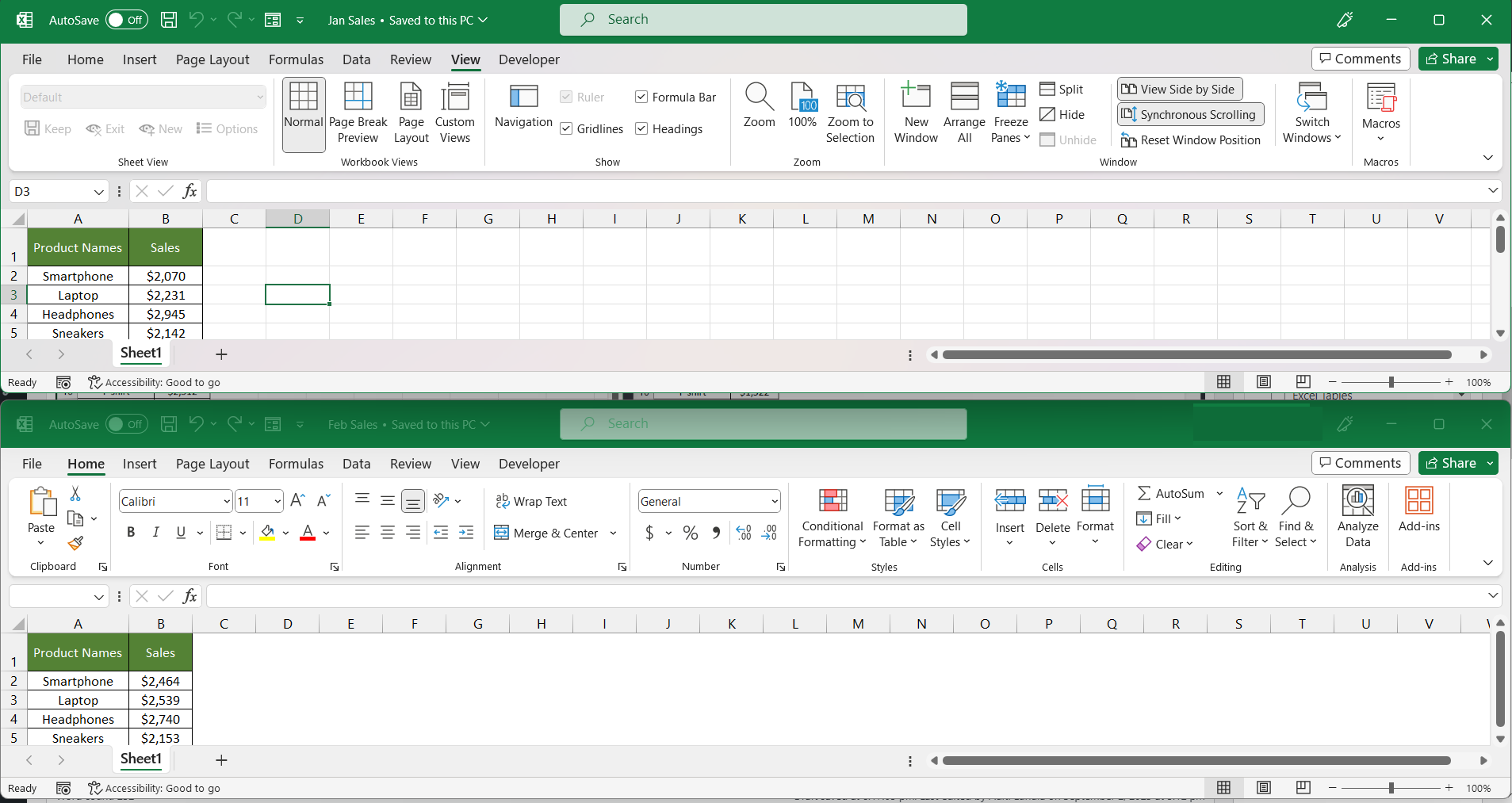
STEP 2: Go to View > View Side by Side.

The two worksheets will be displayed together in the same window horizontally.

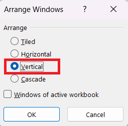
STEP 3: Go to View > Arrange All.

STEP 4: In the Arrange Windows dialog box, select Vertical.

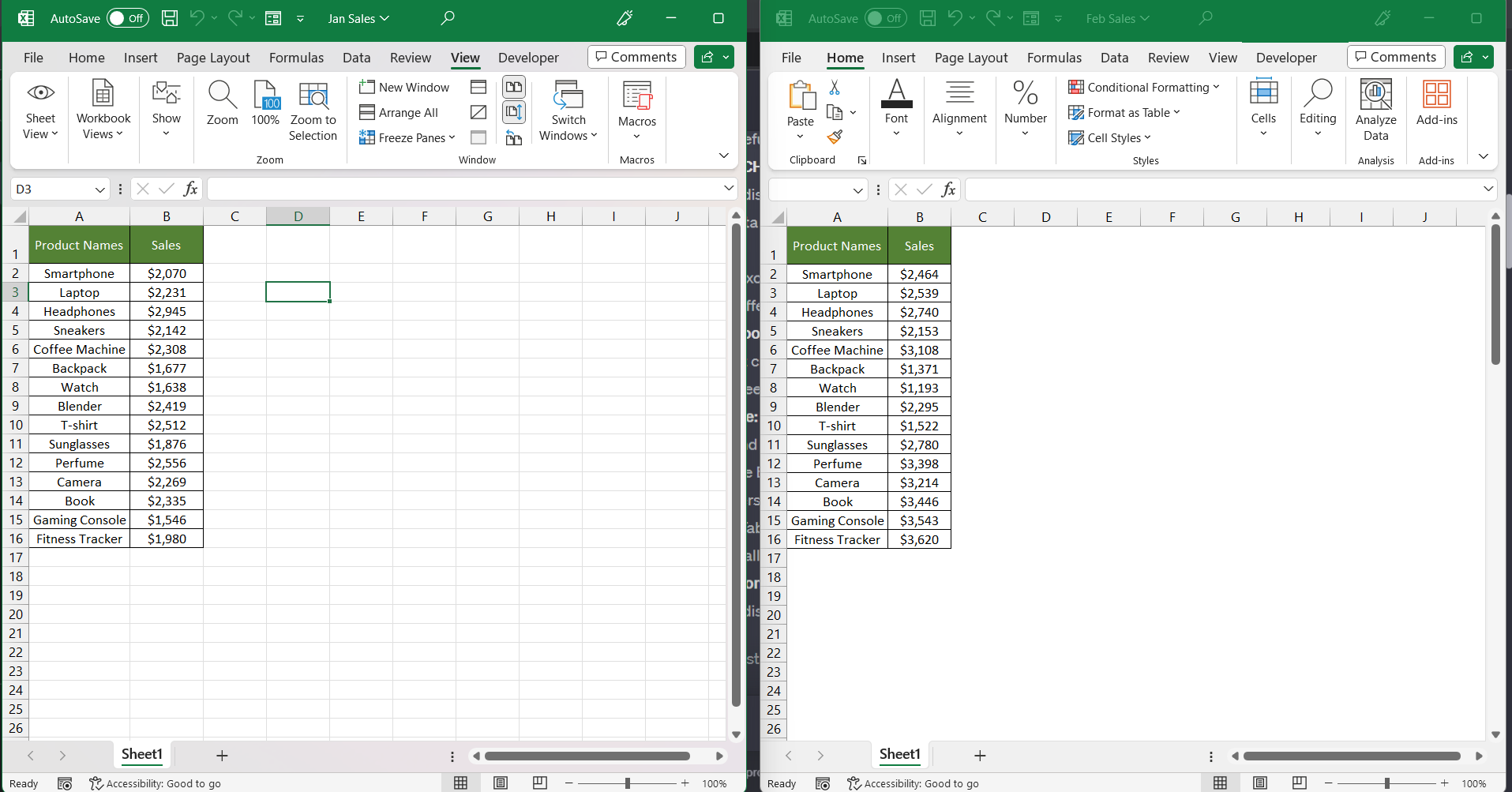
The worksheets will be displayed vertically in the same window.

Now, you can easily compare the sales data in 2 months as they are displayed side by side.

 

#2 – View Side by Side in Same Workbook

If your data is the same workbook but in a different worksheet, even then you can use the view side-by-side option. Follow the steps below to know how –

STEP 1: Open the Excel workbook.

STEP 2: Go to View > New Window.

This will open the same file in a different window.

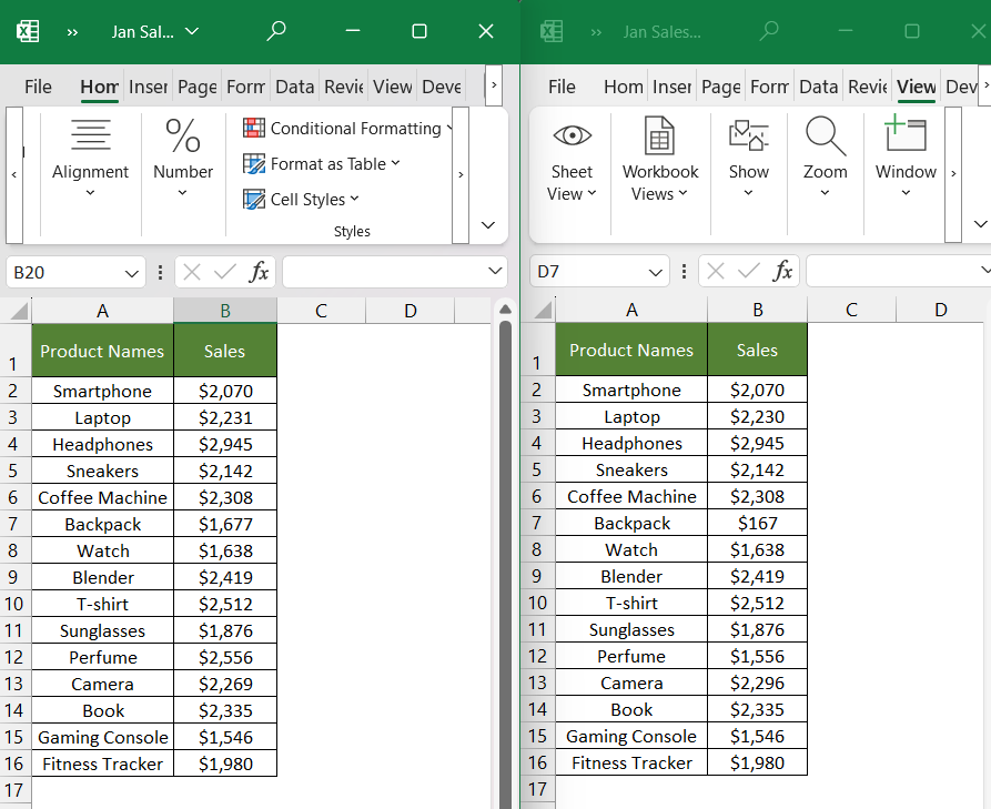
STEP 3: Go to View > View Side by Side.

This will open the same file and it can be viewed side by side.

 

#3 – Compare using Conditional Formatting

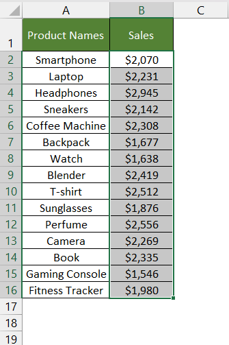
Suppose we have extracted sales data from two different sources and we want to compare if there are any discrepancies between the two. This can be achieved by using conditional formatting and highlighting the differences.

Follow the steps below –

STEP 1: Open the Excel workbook containing the worksheets.

STEP 2: In the sheet where you want to highlight differences, select the cell range where you want the conditional formatting to be applied.

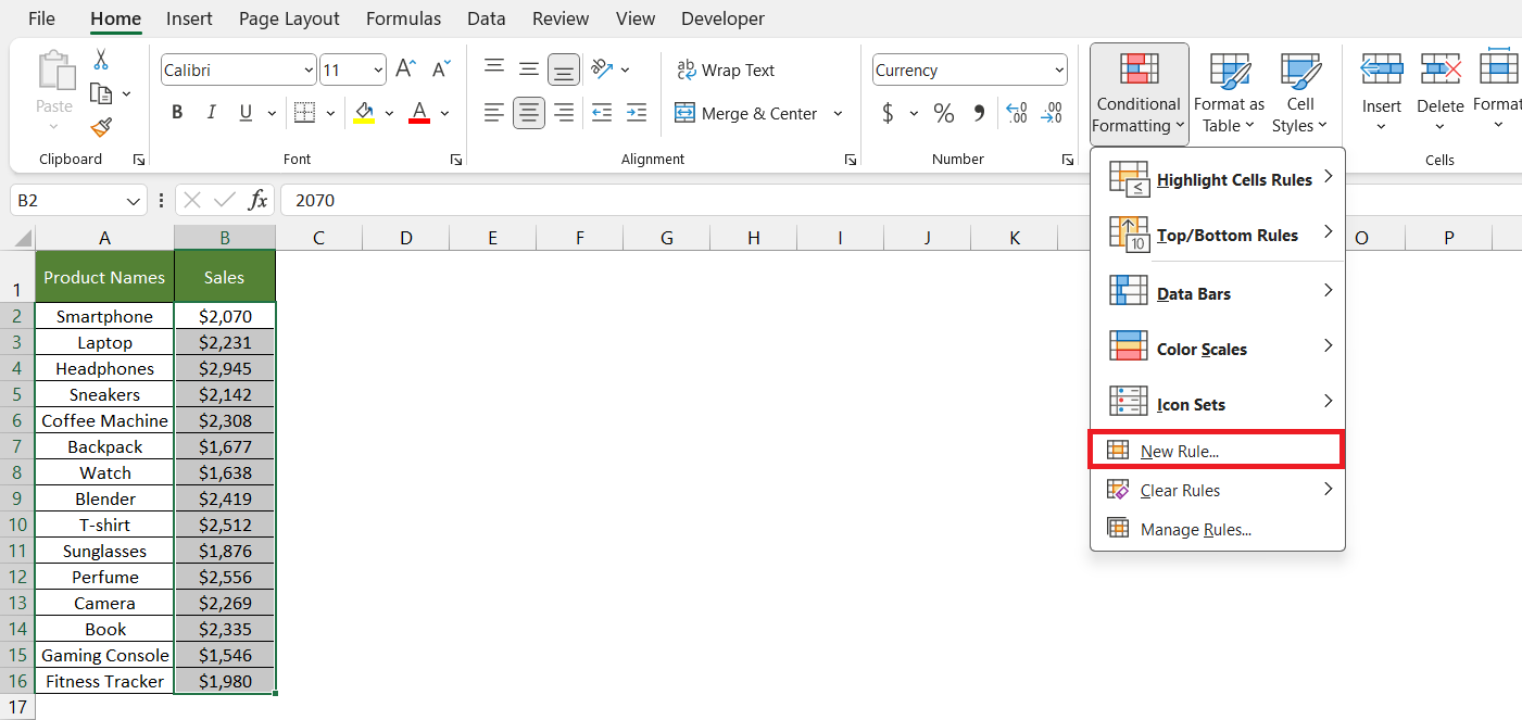
STEP 3: Go to the Home > Conditional Formatting > New Rule.

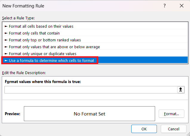
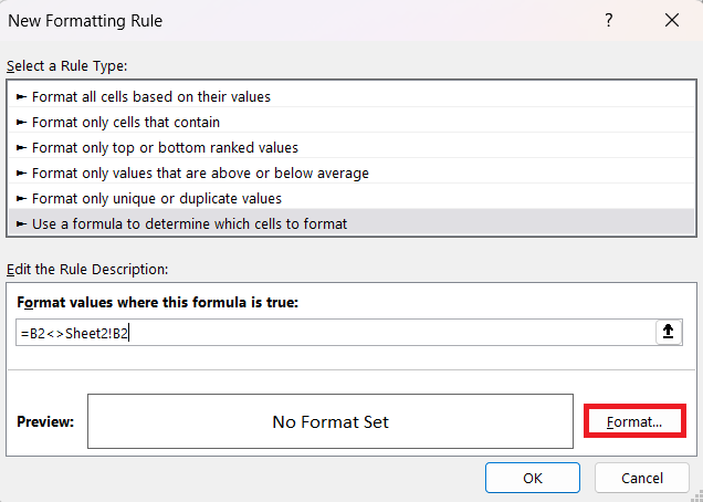
STEP 4: In the New Formatting Rule dialog box, choose Use a Formula to determine which cells to format.

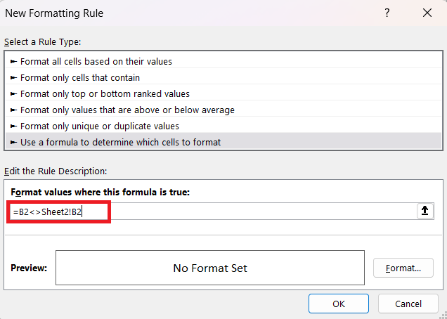
STEP 5: Input the following formula –

=B2<>Sheet2!B2

STEP 6: Click on the Format button.

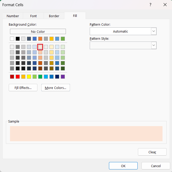
STEP 7: In the Format Cells dialog box, go to the Fill tab. Here, select the light red color that you want to use to highlight the differences and click OK.

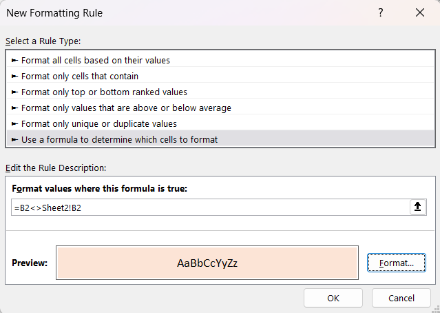
STEP 8: Double-check the result in the Preview section. Click OK.

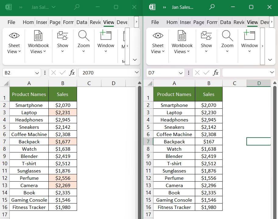
Now, the cell values in Sheet1 that do not match the corresponding cell values in Sheet2 will be highlighted with the selected light red fill color, allowing you to easily spot differences and compare two sheets.

Please Note – This method cannot be used if the data is present in two different workbooks.

 

Conclusion

In Excel, comparing data across different worksheets or workbooks can be a significant challenge. This article discusses three techniques to compare two sheets —View Side by Side in the same or different workbooks and compare using Conditional Formatting.

Whether you need a quick visual comparison or automated highlighting of differences, Excel equips you with the tools to achieve it. We can choose the method that best suits our specific needs and the complexity of the data that we are comparing.

Further learning:

• Stacked Column Chart: Compare Contributions
• Master ANOVA in Excel: A Step-by-Step Tutorial
• 141 Free Excel Templates and Spreadsheets

Click here to understand more about how to view and compare documents.