How to Create Compound Interest Calculator in Excel – 2 Easy Methods

Key Takeaways:

• Flexible Formula Setup: Excel’s basic compound interest formula, =Principal * (1 + Rate/CompoundsPerYear)^(CompoundsPerYear * Years), allows you to calculate future balances based on any initial amount, interest rate, compounding frequency, and time period.
• Incorporating Regular Contributions: By using Excel’s FV function, you can calculate compound interest with additional regular contributions, giving a more realistic picture of savings growth with periodic deposits.
• Building Custom Tables: Excel makes it easy to build a compound interest table to track balances over time. Using a formula across rows, you can see year-by-year growth and adjust for different scenarios to visualize the impact of different compounding periods and rates.

Method 1 – Compound Interest Formula

Suppose you wish to invest $10,000 in your savings account for 3 years. Your account offers a return of 6.5%, subject to semi-annual compounding. You want to know the future value of your investment using the compound interest calculator in Excel.

The formula for this approach will be –

P’ = P*(1+R/N)^NT

where.

• P’ is the future value of the investment, including interest.
• P is the principal amount.
• R is the annual interest rate (in decimal form).
• N is the number of times that interest is compounded per unit t.
• T is the time the money is invested for, in years.

Follow the steps below to learn how to use the compound interest calculator in Excel –

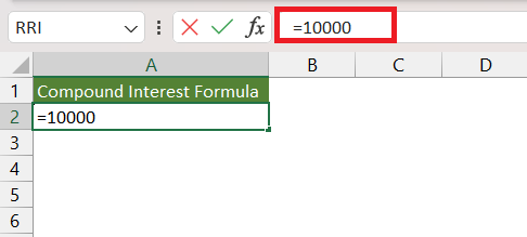
STEP 1: Enter the initial principal amount i.e. P. Here, it is 10000.

=10000

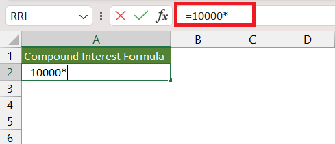
STEP 2: Enter the multiplication sign(*).

=10000*

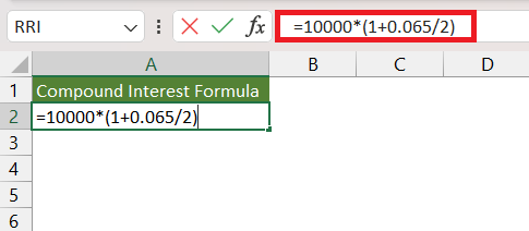
STEP 3: Enter 1 + 0.065/2 within brackets.

=10000*(1+0.065/2)

where,

• o.o65 is the annual interest rate in decimal form i.e. R
• 2 is the number of times the interest is compounded i.e. N

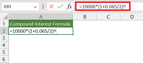
STEP 4: Enter the ^ sign.

=10000*(1+0.065/2)^

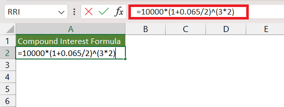
STEP 5: Now, enter the 2*3 within brackets.

=10000*(1+0.065/2)^(2*3)

where

• 2 is the number of times the interest is compounded i.e. N
• 3 is the time the money is invested for i.e. T years.

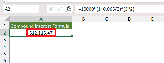
The resultant amount will be the future value of the amount invested, compounded semi-annually.

 

Method 2 – FV Formula

The FV function in Microsoft Excel assists in calculating the future worth of a company’s investments, assuming periodic, consistent payments with a constant interest rate.  Let’s use Microsoft Excel’s FV Function that will help us to create a compound interest calculator in Excel.

The syntax for the FV function is –

=FV(rate,nper,pmt,[pv],[type])

• Rate: The interest rate per period. 
• Nper: The total number of payment periods in an annuity.
• Pmt: The payment made each period. It cannot change over the life of the annuity. Typically, pmt contains principal and interest but no other fees or taxes. If pmt is omitted, you must include the pv argument. 
• Pv: The present value, or the lump-sum amount that a series of future payments is worth right now. If pv is omitted, it is assumed to be 0 (zero), and you must include the pmt argument. Type: This is an optional argument.
• Type: The number 0 or 1 indicates when payments are due. 0 if the amount is being added to the investment at the end of the period or 1 if the amount is being added to the investment at the beginning of the period. This is an optional argument.

Follow the steps below to use the FV function to calculate compound interest –

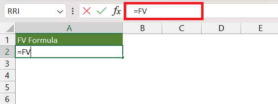
STEP 1: Enter the FV function.

=FV

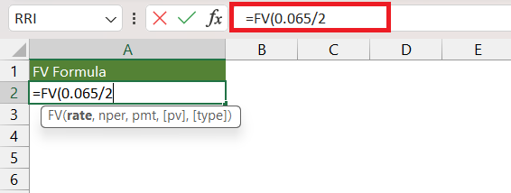
STEP 2: Enter the first argument i.e. rate. Here, it is 0.0065/2 i.e.

=FV(0.065/2

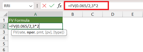
STEP 3: Enter the second argument i.e. nper. Here, it is 3*2 i.e. 6.

=FV(0.065/2,3*2

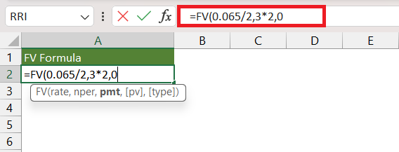
STEP 4: Enter the third argument i.e. pmt. Here, it is 0 as there were no deposits made in between the period.

=FV(0.065/2,3*2,0

STEP 5: Enter the fourth argument i.e. pv. Here, it is -10,000.

=FV(0.065/2,3*2,0,-10000)

You will have to use a negative sign as it is a cash outflow.

The resultant amount is the future value of your investment.

Additional FV Formula Example:

Say that you turn 18 years today (CONGRATS!) and you find out that your parents deposited an amount with their bank when you were born.

Now that you are 18 years old you can collect this money and go spend it all in one day!

How much would be available for you to spend?

Thankfully there is an easy way to calculate this with Excel’s FV formula! FV stands for Future Value.

The future value (FV) is the value of a current asset at a specified date in the future based on an assumed rate of growth over time.

In our example below, we have the table of values that we need to get the compound interest or Future Value from:

(Change the NUMBER OF YEARS column to 18 to see the results on your 18th birthday)

I explain how you can do this below:

STEP 1: We need to enter the FV function in a blank cell:

=FV(

 

STEP 2: The FV arguments:

rate

What is the rate of the interest?

Select the cell containing the interest rate (make sure that this is in a percentage):

=FV(B9,

nper

How many periods?

Select the cell containing the number of years:

=FV(B9, C9,

pmt

What is the periodic payment?

We have no periodic payment, only an initial amount, so let us put in 0:

=FV(B9, C9, 0,

pv

What is the initial amount?

PV stands for present value, the initial amount. We need to change this to a negative value by multiplying -1.

The reason why we need this as a negative value as Excel treats this as “money out” for your investment.

=FV(B9, C9, 0, A9 * -1)

 

Apply the same formula to the rest of the cells by dragging the lower right corner downwards.

You now have all of the compound interest results!  GO OUT & SPEND!

Frequently Asked Questions:

How do I calculate compound interest in Excel?

You can calculate compound interest using the formula:
=Principal * (1 + Rate/CompoundsPerYear)^(CompoundsPerYear * Years)
Replace Principal with your initial investment, Rate with the annual interest rate (as a decimal), CompoundsPerYear with the number of times interest is compounded per year, and Years with the total duration in years.

Can I calculate compound interest with periodic contributions in Excel?

Yes, you can use the Future Value (FV) function to include regular contributions:
=FV(Rate/CompoundsPerYear, CompoundsPerYear * Years, -Contribution, -Principal, 1)
Here, Contribution is your regular deposit, and Principal is the initial amount. Setting the last parameter to 1 calculates the future value with contributions at the beginning of each period.

How can I build a compound interest table for each year?

To create a yearly breakdown, enter your initial balance in the first cell, then use a formula in subsequent cells that compounds the interest based on the previous year’s balance. For example, in cell B2, use =B1*(1 + Rate/CompoundsPerYear) and copy it down for each year to see the balance grow annually.

Conclusion

In conclusion, understanding and utilizing compound interest calculator is crucial for maximizing returns on investments over time. By employing either the Compound Interest Formula or the FV Formula in Excel, investors can project the future value of their investments more accurately.

These tools empower individuals to make informed financial decisions and harness the power of compound interest for long-term financial growth.

Click here to learn more about Finance Formulas in Excel.