How to Concatenate Cells and Strings in Excel – Step by Step Guide

Delve into the realm of Microsoft Excel‘s CONCATENATE function, where separate strings of text are seamlessly woven into a single coherent strand. This function, designed for merging text strings, maintains structure and enhances readability in Excel spreadsheets, reducing clutter effectively.

Key Takeaways:

• Simplicity with CONCATENATE: Merge text strings effortlessly, maintaining spreadsheet structure and enhancing readability.
• Ampersand Magic: Utilize the “&” symbol to combine text and cells swiftly, perfect for including fixed text within the combined result.
• Efficiency with CONCAT and TEXTJOIN: Concatenate cell ranges or customize delimiters swiftly using CONCAT and TEXTJOIN functions, saving time and manual entry fuss.
• Addressing Common Pitfalls: Overcome issues like table expansion errors and formatting challenges with line breaks or delimiters using advanced techniques.
• Creative Fusion with Functions: Combine CONCATENATE with other Excel functions for dynamic formulas, transforming and presenting data effectively.

 

Introduction to Concatenation in Excel

Understanding the CONCATENATE Function

Diving into the world of Excel, you might find yourself needing to weave separate strings of text into a single coherent strand. That’s where the CONCATENATE function steps in to save the day. It’s a text function designed specifically for this purpose, allowing you to merge two or more text strings seamlessly.

The beauty of this function lies in its simplicity: with it, your Excel spreadsheets can maintain structure, enhance readability, and reduce clutter by consolidating information effectively.

Step-by-Step Guide on Concatenating Cells

Unleashing the full potential of the CONCATENATE function is like mastering a secret Excel spell. To get started, pick the cells you want to merge and type “=CONCATENATE(” followed by the cell references, separating each with a comma. Hit enter, and voila! The cells blend like a culinary masterpiece.

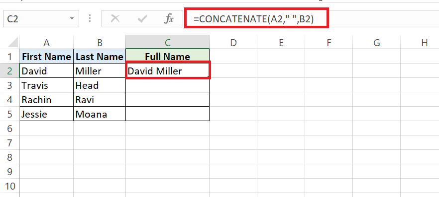
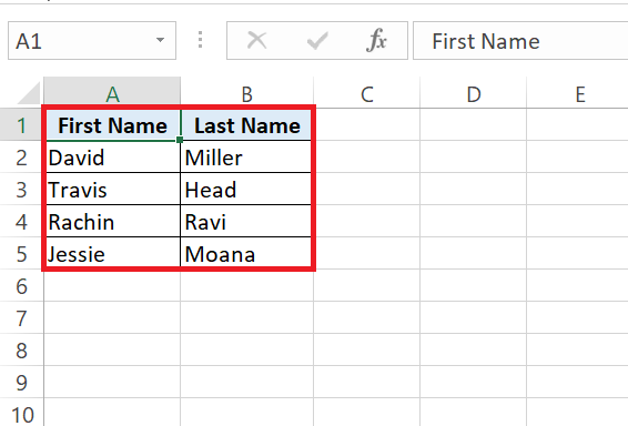
Consider a list with first names in column A and last names in column B. To craft full names in column C, your formula might look like “=CONCATENATE(A2, ” “, B2)”. Notice the space (” “) added as a text argument? It ensures that your final text won’t be a jumble of characters but rather a neatly spaced combination.

STEP 1: In cell C2, enter the formula “=CONCATENATE(A2, ” “, B2)” to combine the first and last names with a space in between.

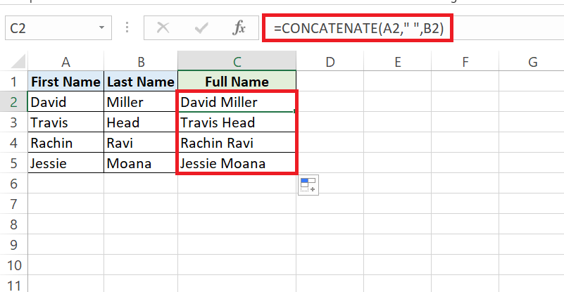
STEP 2: Drag the formula down to apply it to all rows in the dataset.

Enjoy the magic of CONCATENATE for seamless text merging in Excel!

Combining Text and Cells with “&

When it comes to Excel wizardry, combining text and cells using the ampersand (“&”) is like finding a shortcut on a long road. Start with “=”, click on the cell you wish to combine, type “&”, and then type or select the next part—repeat as needed. This approach is especially handy when you want to include fixed text—like labels or separators—within your combined result.

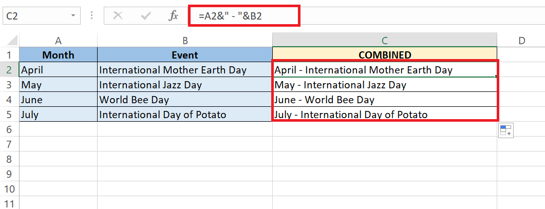
Let’s say you’ve got dates in one column and event names in another. To craft a detailed narrative in a third column, your formula could be a simple “=A2&” – “&B2”.

STEP 1: In cell C2, enter the formula “=A2&” – “&B2” to combine the date and event names with a dash in between and press enter.

STEP 2: Drag the formula down to apply it to all rows in the dataset.

It weaves in a dash between the date and event for an instant, clear report. No need for any heavyweight function, just an agile ampersand doing the heavy lifting.

 

Tips on Concatenating Multiple Ranges and Strings

The CONCAT Function for Range Concatenation

If your data spans across multiple cells in a range, say hello to the CONCAT function. This gem allows you to concatenate a range of cells quickly without typing each cell reference individually. Think of it as the CONCATENATE function but with a power-up for handling arrays more efficiently.

Just type “=CONCAT(” and select your desired range. No more separating each cell with a comma—Excel does the heavy lifting. For instance, “=CONCAT(A1:A10)” would seamlessly stitch together text from ten cells in column A, transforming a list into one continuous string. It’s perfect for times when you’re looking to combine large chunks of data without manual entry fuss.

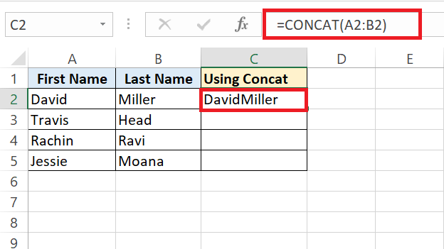
STEP 1: Prepare your dataset with the text you want to concatenate across multiple cells in a range.

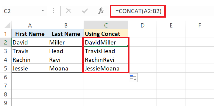
STEP 2: In a blank cell C2, enter the formula “=CONCAT(” and select the range of cells you want to combine. Press Enter and Excel will automatically concatenate the text from the selected cells into one continuous string.

STEP 3: Drag the formula down to apply it to all rows in the dataset.

 

Handy Tricks with the TEXTJOIN Function

The TEXTJOIN function is where Excel really shows off its flexibility in concatenation. This function stands out by offering two significant trump cards: You can define a delimiter to neatly separate combined texts, and choose to skip over any blank cells in your range.

Picture needing to join a cluster of names, but some cells are empty. With TEXTJOIN, you set “=TEXTJOIN(“,”, TRUE, A1:A5)”, and the function smartly skips the blanks, leaving you with a comma-separated list that’s clean and professional.

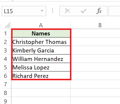
STEP 1: Organize your dataset with names in cells A2 to A6.

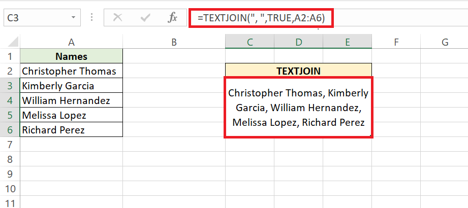
STEP 2: In a blank cell, enter the formula “=TEXTJOIN(“, “, TRUE, A2:A6)” to concatenate the names with a comma as a delimiter, skipping over any blank cells. Press Enter, and you’ll get a clean, comma-separated list of names without any empty cells disrupting the output.

It’s particularly a game-changer when you’re dealing with data that’s not consistently filled in and you want to maintain a clean output.

Common Concatenation Pitfalls and How to Avoid Them

Issues When Expanding Named Tables

When you’re working with named tables in Excel, sometimes expanding them after using concatenation can lead to a few hitches. If you’ve set up a table that uses concatenation, and you want to add more rows, Excel might not always auto-fill your formulas correctly. This can result in #REF! errors or incorrect data being shown.

To avoid these issues, always ensure that any concatenation formulas are correctly referencing the table columns. Use structured references like TableName[ColumnName] within your formulas.

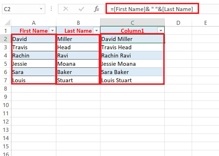
STEP 1: In a blank column cell C2, enter the formula “==[First Name]& ” “&[Last Name]” to concatenate the names.

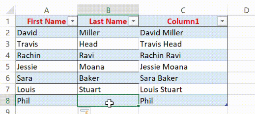
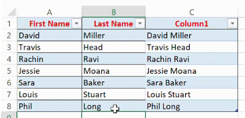
STEP 2: As you add more rows to the table, Excel will automatically extend the formula to include the new data, maintaining accuracy.

Once we complete the First and Last Name, the formula is extended automatically to it as well.

 

NOTE: Ensure all concatenation formulas reference table columns using structured references to avoid #REF! errors or incorrect data.Keep your data tidy and error-free by using structured references in concatenation formulas within named tables.

This way, as you add more rows, Excel knows to extend the formulas using the same structure you’ve originally set up, keeping your data tidy and error-free.

Solving Problems with Line Breaks and Delimiters

Merging different data into one cell and maintaining a clean structure often requires using line breaks or specific delimiters, especially with addresses or lists. Here’s where some might hit a snag because typing a line break into a formula isn’t straightforward.

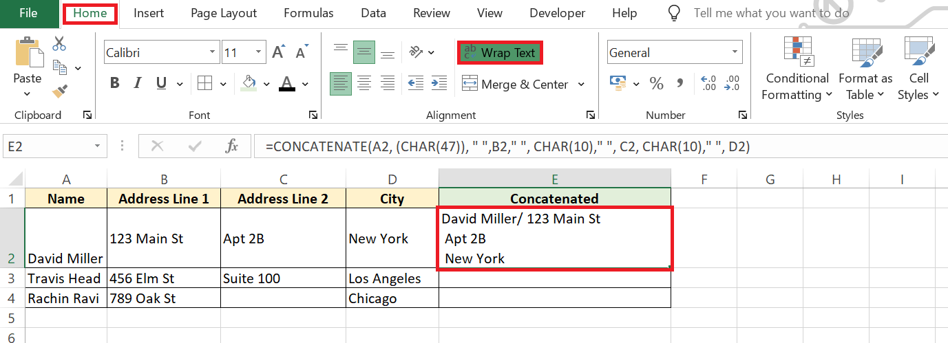
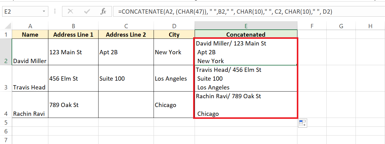
The solution lies in Excel’s CHAR function. To insert line breaks on Windows, use CHAR(10), while on Mac, you’ll want to use CHAR(13) within your CONCATENATE or TEXTJOIN formulas. Remember to check the “Wrap text” option in the cell format settings to ensure the line breaks actually display.

STEP 1: In a blank cell E2, enter the formula “=CONCATENATE(A2, (CHAR(47)), ” “,B2,” “, CHAR(10),” “, C2, CHAR(10),” “, D2)” to merge the address lines with line breaks. And enter the formula.

STEP 2: Select the cell, go to the “Home” tab, and click on the “Wrap Text” button to ensure line breaks display correctly.

STEP 3: Drag the formula down to apply it to all rows in the dataset. With CHAR(10) for line breaks, (CHAR(35)) for slash and wrap text enabled, you can neatly merge address data in Excel.

For delimiters other than line breaks, CHAR comes to the rescue again, enabling characters like double quotes (CHAR(34)), slashes (CHAR(47)), or other special characters. Armed with this knowledge, you’ll turn what could be a concatenation headache into no problem at all.

Advanced Techniques for Data Combination in Excel

Merging Columns Row-by-Row Intelligently

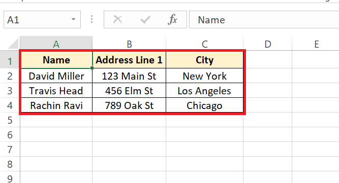
When your goal is to merge entire columns row-by-row, you’re looking for an intelligent approach where no data gets lost. Merging columns in Excel can be child’s play with the right techniques. Suppose you’re working with three columns of data; the strategy is to use a formula that will concatenate the cells of each row across those columns, while placing a delimiter of your choice in between.

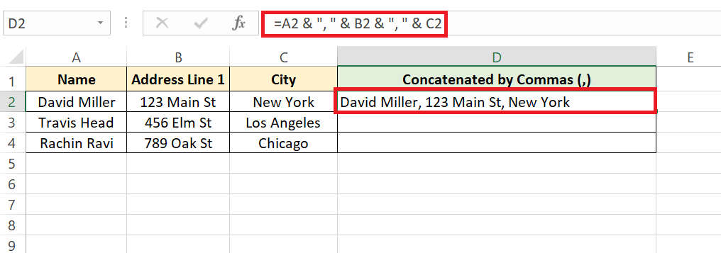
An effective way to do this is by using the “&” or CONCAT function, placed in the row where you want your results to begin. For example, the formula “=A2 & “, ” & B2 & “, ” & C2″ merges the data from columns A, B, and C with a comma and space acting as delimiters between data points. Then, simply drag the formula down the rows to apply it to the entire column. After that, you’ve got your data combined into one tidy and easy-to-read top row.

STEP 1: Create a new dataset with columns for data, e.g., “Column A”, “Column B”, and “Column C”.

STEP 2: In the top row of a new column, enter the formula “=A2 & “, ” & B2 & “, ” & C2″ to concatenate data from each row with a delimiter, like a comma and space.

STEP 3: Drag the formula down to apply it to all rows in the dataset, combining the data into one tidy column. Now, each row’s data from the specified columns is merged into a single, easy-to-read column.

 

Creative Uses of CONCATENATE with Functions

Sometimes in Excel, you’re not just merging data—you’re transforming it. CONCATENATE can play well with other functions to create more dynamic and useful formulas. Want to combine text strings with dates while keeping the date format intact? Pair CONCATENATE with the TEXT function. It lets you maintain date formatting by specifying how you want the date to appear.

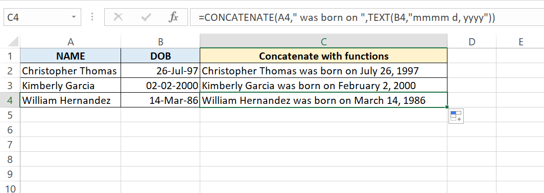
Let’s say you want to join a person’s name with their birthday. The formula “=CONCATENATE(A1, ” was born on “, TEXT(B1, “mmmm d, yyyy”))” will yield a sentence with the full date in a friendly, readable format. Or perhaps you’re dealing with currency values? No worries, CONCATENATE can blend those in too, ensuring that your financial data is clearly communicated with appropriately formatted figures.

STEP 1: Create a new dataset with columns for names (Column A) and birthdates (Column B).

STEP 2: In a new column, enter the formula “=CONCATENATE(A2, ” was born on “, TEXT(B2, “mmmm d, yyyy”))” to merge names with birthdates while preserving date format.

STEP 3: Drag the formula down to apply it to all rows in the dataset. Now, each row will display a sentence with the person’s name and birthdate in a friendly format.

FAQs

What Exactly is “Concatenate” in Excel?

In Excel, “concatenate” is a fancy term for linking or joining together. This means combining the text from different cells into one cell without altering the original values. It’s a nifty way to merge data like names and addresses or wrap up bits of information into a neat package, all while keeping your original data untouched.

Can You Concatenate a Range of Cells?

Absolutely, concatenating a range of cells is a breeze in Excel. Whether you’re using the CONCAT or TEXTJOIN function, you can reference an entire range, like A1:A10, and merge the content of those cells swiftly. It’s a time-saver when you’re tasked with combining lengthy lists or numerous data points into a single cell.

What Are the Alternatives to the CONCATENATE Function?

The go-to alternatives to the CONCATENATE function are the CONCAT and TEXTJOIN functions. CONCAT is like a more modern sibling to CONCATENATE, handling ranges with less fuss. TEXTJOIN steps it up a notch, allowing for delimiters and skipping empty cells. Let’s not forget the simple ampersand (“&”), a quick-fire way to link text strings without a full-fledged function.

How to Concatenate Cells with Different Delimiters?

To concatenate cells with various delimiters in Excel, you can mix and match within your formula. Whether you’re partial to commas, semicolons, or spaces, you wrap the character in quotes and place it between cell references using either the CONCATENATE function, the ampersand (“&”), or the TEXTJOIN function, which is explicitly designed to insert custom delimiters as you merge cells.

How do I CONCATENATE two columns in Excel?

To concatenate two columns in Excel, simply use the CONCATENATE function or the ampersand (“&”) in the cell where you want to display the combined data. If you have values in columns A and B, input “=CONCATENATE(A2, ” “, B2)” or “=A2 & ” ” & B2″ for a space between the merged data. Drag the corner of the cell downwards to apply this to the entire column.