Quick Excel Guide: Conditional Format Blank Cells

Conditional formatting in Microsoft Excel is a powerful tool to visually differentiate and emphasize data based on specific criteria, such as conditional format blank cells. Despite its apparent simplicity, applying conditional formatting to blank cells can be complex, as Excel’s interpretation of ‘blank’ may not always align with user expectations. This intricate feature allows users to swiftly locate and manage empty entries, enhancing both data analysis and accuracy.

Key Takeaways

• Excel’s Conditional Formatting visually guides users to automatically format cells based on specified criteria, enhancing data analysis.
• Distinguish truly blank cells from those with invisible characters for accurate data analysis and reliability in Excel workbooks.
• Quickly identify missing data with a simple guide for highlighting blank cells using conditional formatting, making data gaps visually apparent.
• Users can create custom formulas like ISBLANK for precise blank cell detection, offering versatility in cell selection and formatting.
• Utilize VBA Macro for enhanced control in highlighting blank cells.

Download the Excel Workbook and follow along to understand how to conditional format blank cells in Excel – Download excel workbookConditional-Format-Blank-Cells-in-Excel.xlsm

 

Introduction to Conditional Formatting in Excel

The Basics of Conditional Formatting

Conditional Formatting in Excel is like the traffic lights of a dataset—it guides you where to pay attention. It is a handy tool that allows you to automatically apply a format to a cell or a range of cells based on certain criteria. This could be anything from a simple color fill to data bars and color scales, helping you visualize data at a glance.

Importance of Differentiating Blank vs. Non-Blank Cells

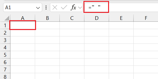
Understanding the difference between blank and non-blank cells in Excel is crucial for accurate data analysis. While both types of cells might appear empty, only truly blank cells contain no data whatsoever. Cells that may look blank could hold invisible characters, like spaces or formulas returning empty strings, which can skew your results and calculations. By differentiating them correctly, you ensure the integrity of your data and make your Excel workbooks more reliable and error-proof.

 

Step-by-Step Guide to Conditional Format Blank Cells

Highlighting blank cells can make your spreadsheet more intuitive and helps to quickly identify where data may be missing. Here’s a step-by-step guide to conditional format blank cells:

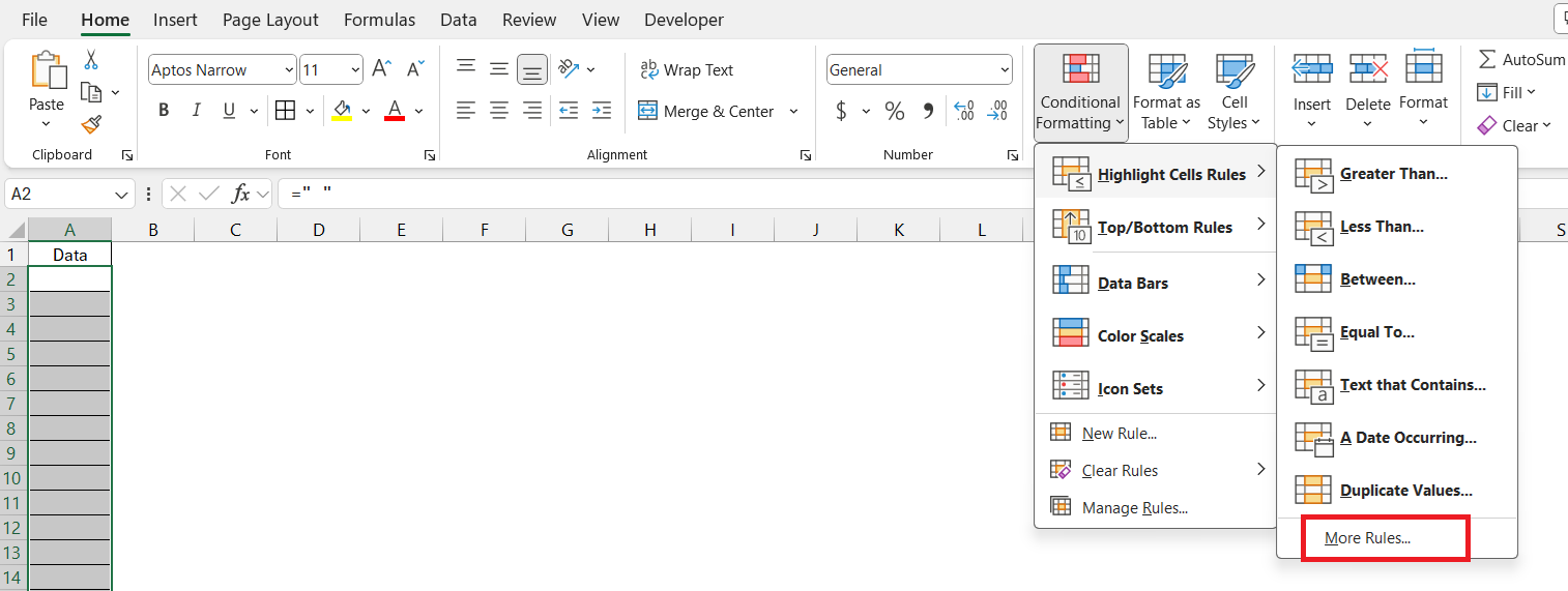
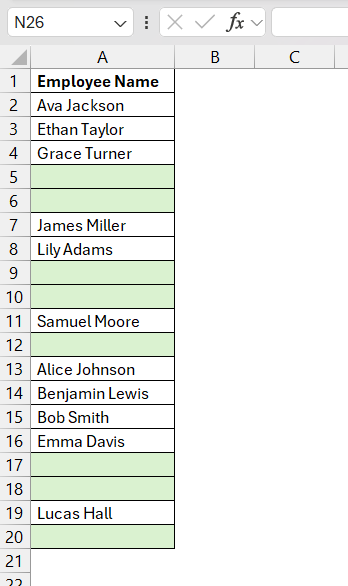
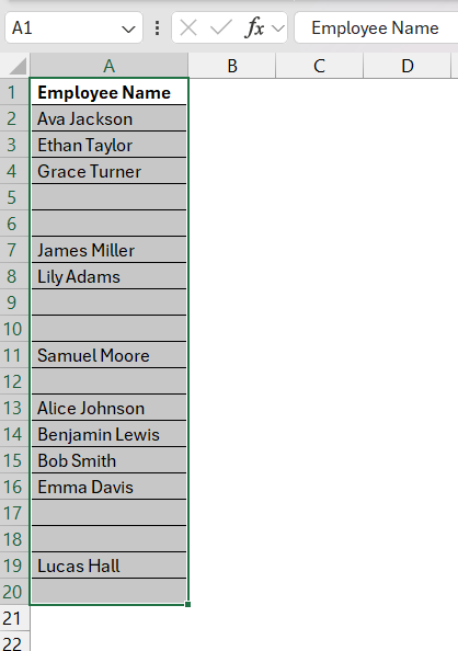
STEP 1: First up, select the range where you suspect there are blanks. Suppose you choose A2:A20.

STEP 2: Head to the ‘Home’ tab and find the ‘Styles’ group. Click on ‘Conditional Formatting.

STEP 3: Go to ‘Highlight Cells Rules‘ followed by ‘More Rules.

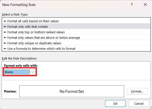
STEP 4: In the new window, opt for ‘Format only cells that contain’, then pick ‘Blanks’ from the drop-down list.

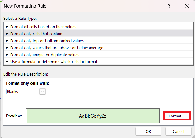
STEP 5: Now, click on the Format button to select the formatting style of your preference, maybe a nice fill or text color to stand out.

STEP 6: Hit ‘OK’, and voilà! All blank cells in your selected range will now be visually distinguished.

This nifty feature does not just make for a color-filled spreadsheet, but it makes any gaps in data instantly obvious.

 

Custom Formulas for Blank Cell Detection

Sometimes the standard blank cell options in Excel’s conditional formatting are not enough. For those occasions, you can write custom formulas to suit your unique needs. Let’s get into how you can craft these formulas:

STEP 1: Select the range you’re working with (for instance, A2:A20).

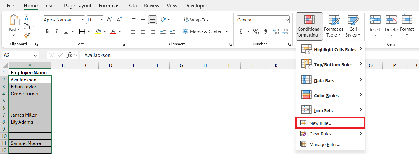
STEP 2: Go to the ‘Home’ tab and click ‘Conditional Formatting’, followed by ‘New Rule’.

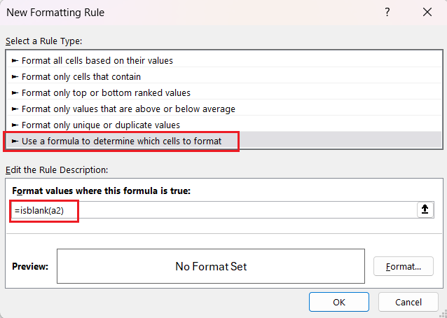
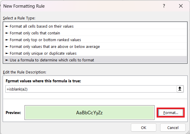
STEP 3: Choose ‘Use a formula to determine which cells to format’. In the formula box, type in =ISBLANK(A2) to highlight truly blank cells.

STEP 4: After entering your formula, hit the ‘Format…’ button to choose the visual style you want to apply.

STEP 5: Click ‘OK’ to set the rule.

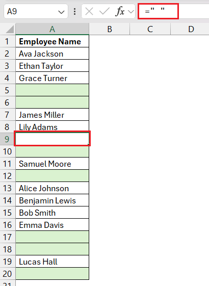
This method is useful if you want to capture cells that may look blank but could contain invisible characters such as spaces. These custom formulas offer versatility in how you select and format cells, allowing for precise and contextual conditional formatting that extends beyond built-in options.

 

Troubleshooting Common Issues

Why Blank Cells May Not Be Highlighted

If you’ve attempted the steps to highlight blank cells and haven’t seen the results you’re expecting, a few culprits could be at play:

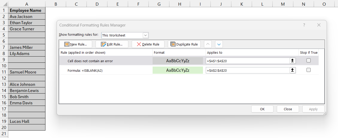
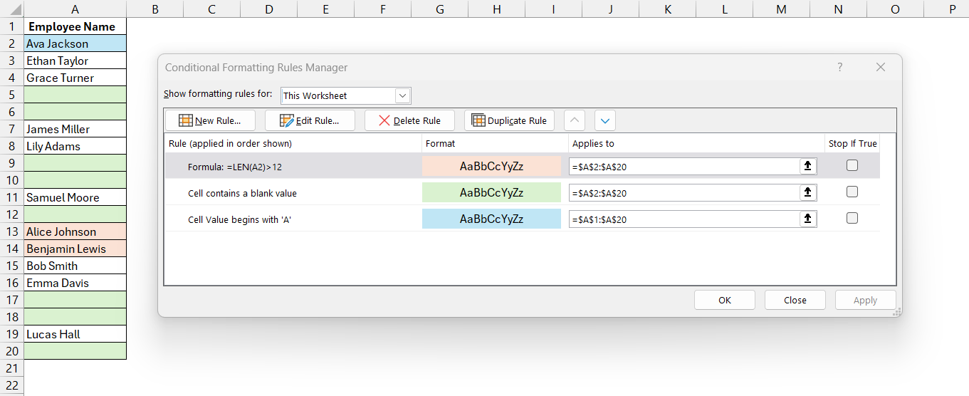
• First-in Priority Rule: Sometimes, the order of conditional formatting rules interferes with how they are applied, especially if existing rules affect the same cells.

• Incorrect Formula: A formula may have syntactical errors, be ill-suited for the task, or incorrectly reference cell ranges or types.
• Cell Content: Cells that seem empty but contain spaces, formulas that output nothing, or even cells with font color matching the background, may be mistaken as non-blank.

To triumph over these tricky situations, always check the formula you input for accuracy carefully, ensure that the cells are truly empty, and revisit rule precedence to make sure the blank cell formatting rule is appropriately prioritized.

 

Solving Unintended Highlights of Non-Blank Cells

If you’ve unintentionally highlighted cells that aren’t blank, don’t worry; it’s a common hiccup in Excel that can be easily fixed. Here’s how:

• Review Your Data: Double-check that the cells don’t contain any hard-to-see data like spaces, very small text, or font color matching the background.
• Check the Formulas: If the cells contain formulas that return an empty string, they will be treated as non-blank. Adjust the formula or the conditional formatting rule to account for this.
• Inspect Conditional Formatting Rules: Navigate to ‘Manage Rules’ under the Conditional Formatting options and ensure that the rules are set correctly, without overlaps that might cause confusion.

Once you’ve made the appropriate adjustments, your highlight should accurately reflect truly blank cells, making your data much easier to manage and interpret.

 

Advanced Tips and Tricks

Using VBA for Enhanced Blank Cell Formatting

For those who love to streamline tasks in Excel, Visual Basic for Applications (VBA) can give you more control and flexibility, especially with tasks like highlighting blank cells. Here’s a concise guide for using VBA for blank cell detection:

STEP 1: Press ALT + F11 to open the Developer tab and access the Visual Basic Editor.

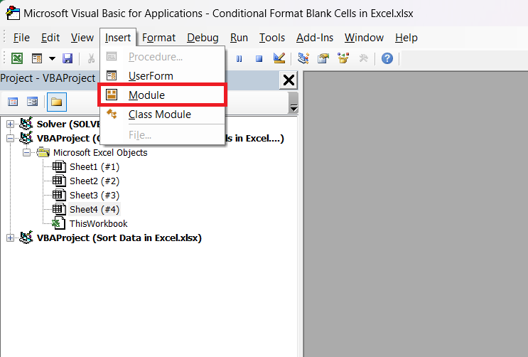
STEP 2: Insert a new module by clicking ‘Insert’ > ‘Module’.

STEP 3: Paste the following VBA script into the module:

STEP 4: Close the VBA Editor and go back to Excel.

STEP 5: Select the range where you want to highlight blank cells.

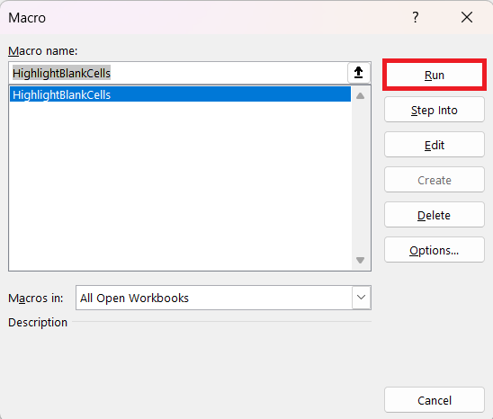
STEP 6: Press ALT + F8, select ‘HighlightBlankCells’, and click ‘Run’.

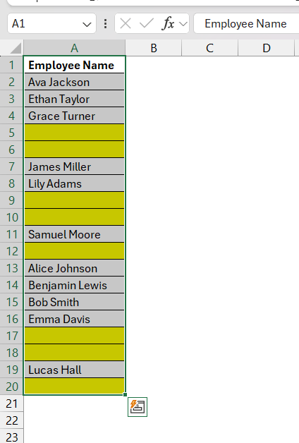
This VBA approach lets you customize the highlighting color and even the criteria for what is considered ‘blank’.

It’s a powerful way to enhance your worksheets, particularly if you need to apply special logic or automate processes.

 

Combining Conditional Formats for Data Analysis

Combining different conditional formats opens up a world of possibilities for data analysis in Excel. This approach allows you to layer multiple criteria to paint a vivid picture of the data landscape. Here’s how to marry various conditional formats effectively:

1. Begin by setting a basic conditional format, such as highlighting blank cells, as previously outlined.
2. Keeping the same data range selected, add a new rule under ‘Conditional Formatting’ to mark cells that surpass a certain numerical threshold or match specific text criteria.
3. Continue layering additional rules as needed. For example, apply a second condition to shade cells that contain values below the average.
4. Excel will apply these rules in the order they are listed, so you can use the ‘Manage Rules’ function to rearrange them for your desired visual effect.

By combining formats, you can, for instance, identify blank cells that are meant to contain pivotal data or discover cells that deviate from the expected range, ensuring a comprehensive insight into your dataset.

 

Practical Applications and Examples

Improving Data Entry Accuracy

Employing conditional formatting for blank cells significantly improves data entry accuracy in Excel. It provides an immediate visual cue, prompting users to fill in necessary information—or perform a double-check—thereby reducing errors and omissions.

Benefits include:

• Immediate Visibility: Highlighted blank cells can be spotted instantly, allowing for quick correction or completion.
• Data Entry Guidance: For larger datasets, color-coded cells guide users systematically through the required data input process.
• Error Reduction: The chances of inadvertently skipping essential fields are decreased.

By integrating conditional formatting into your data entry workflows, you ensure that the data collected is comprehensive and reliable, simplifying subsequent data analysis and enhancing overall decision-making processes.

Streamlining Project Management with Conditional Formatting

Conditional formatting can be an invaluable asset in streamlining project management tasks in Excel. It allows project managers to easily track progress, identify overdue tasks, and analyze resource allocation, all at a glance.

Here’s how it can be leveraged:

• Task Status: Assign colors to categorize tasks as ‘Not Started’, ‘In Progress’, or ‘Completed’. This simplifies the monitoring process of various project stages.
• Deadline Alerts: Highlight impending due dates or overdue tasks with contrasting colors, prompting immediate action.
• Resource Utilization: Use color scaling to identify which team members are under or overutilized based on the volume of tasks assigned.

With conditional formatting doing the heavy lifting, project management becomes a more visual and dynamic experience, enhancing efficiency and keeping everyone aligned.

 

FAQ Section

What is the shortcut to highlight blank cells?

There isn’t a direct keyboard shortcut for highlighting blank cells in Excel, but you can use a combination of shortcuts. Press F5 to open the “Go To” dialog box, then Alt + S to hit the “Special” button, followed by x to select “Blanks”, and then OK.

How Do I Apply Conditional Formatting to Multiple Sheets at Once?

To apply conditional formatting to multiple sheets simultaneously in Excel, you’ll have to group the sheets by selecting them while holding the Ctrl key (Cmd key for Mac). Once grouped, apply conditional formatting to the active sheet, and the same rule will be applied to all selected sheets in the group.

How Can I Extend Conditional Formatting Rules Across an Entire Row or Column?

To extend conditional formatting across an entire row or column based on a specific cell’s value, you use a formula in the conditional formatting rule. For rows, select your range and use a formula like =$A1="" if you’re basing the format on column A. For columns, it would be =A$1="". This locks the reference column or row and applies the format across the entire row or column where the condition is met.

What is the formula for identifying blank cells in Excel?

In Excel, the formula to identify blank cells using conditional formatting is typically written as =ISBLANK(A1), with A1 being the reference to the top-left cell in the selected range. This formula checks if the cell is empty and can be used to trigger conditional formatting rules that highlight or take action on blank cells within a dataset.