How to Use Conditional Formatting Based on Another Cell

Key Takeaways:

• Creating Dynamic Rules: You can apply conditional formatting to a cell based on the value of a different cell, making it easy to highlight data dynamically. For example, set formatting in cell B1 based on the value in cell A1 to visually track dependencies.
• Using Custom Formulas: With custom formulas, you can create flexible rules that apply formatting based on complex criteria. For instance, use =A1>100 in conditional formatting to highlight cells when the referenced cell exceeds a certain value.
• Improving Data Visualization: Conditional formatting based on other cells helps make relationships and patterns more apparent, especially in large datasets. It’s useful for creating interactive dashboards or visually comparing related data across rows and columns.

 

Our final product will look like this:

In this example, we want to highlight the name of the students in column A who have a mark above 80 on column C, indicating their passing status.

Let’s go through these steps thoroughly!

Based on One Cell

The first step is to create your new conditional formatting rule.

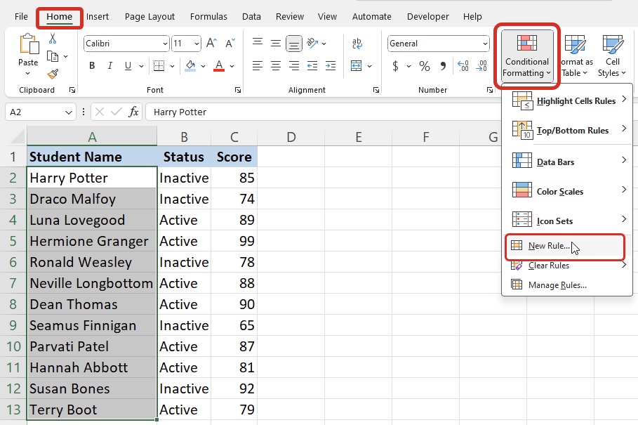
Highlight the range of names from A2 to A13.

Go to the Home tab and click on Conditional Formatting.

Select New Rule.

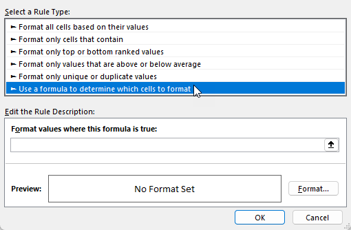
Click on Use a formula to determine which cells to format.

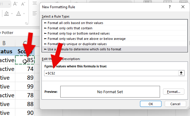
Under the Format values where this formula is true, type in the = sign and click on C2.

As you can see, Excel will automatically consider cell C2 as an absolute reference as it put the $ sign in front of both column C and row 2. To allow this formula to copy down to the other rows, it is important for us to delete the $ sign in front of row 2 to make it a relative reference.

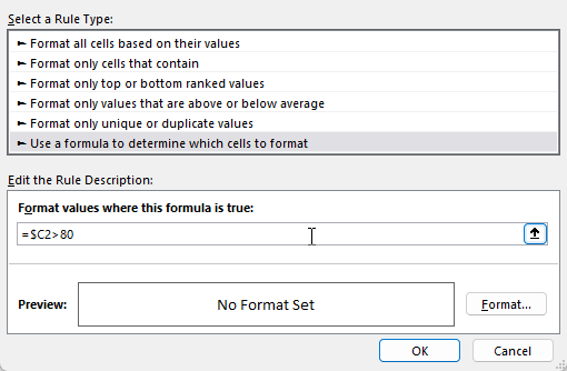
Type in the final formula as =$C2>80.

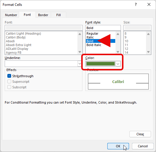
Click on Format to decide on how you want the names that meet the condition to look. You can modify the cells based on font color, background color, borders, and other formatting choices. In our example, we will select bold and the color green. Click OK.

As you can see, the names of the students in column A are highlighted based on their passing score on column C.

Bonus: Formatting Based on Multiple Cells

What if we wanted to highlight cells based on multiple conditions from multiple cells?

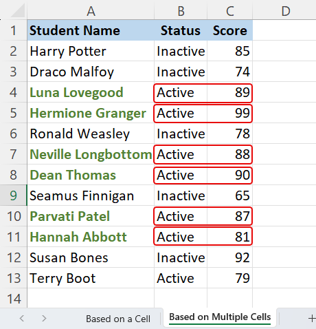
Let’s say we only want to highlight the student names in Column A if their status in Column B is Active AND their score in Column C is higher than 80.

Select the range.

Go to the Home tab and click on Conditional Formatting.

Select New Rule.

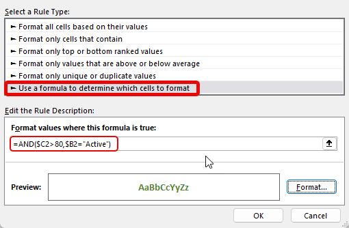
Click on Use a formula to determine which cells to format.

Enter the formula =AND($C2>80, $B2=“Active”). This formula is basically saying we want to format values where this formula is true if the cell in column C is greater than 80 AND if the cell in column B is active.

Choose the Format you would like the cells to be in and click OK.

As you can see, only the names of the students in column A are highlighted based on their passing score above 80 in column C and their active status in column B.

Troubleshooting Common Conditional Formatting Issues

Resolving Conflicts Between Multiple Rules

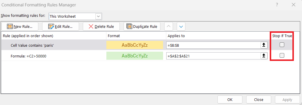
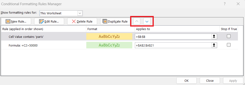
When you’re neck-deep in organizing that dataset in Excel and the colors won’t align to your logic, it might be due to conflicting rules. To get to the bottom of this, you’ll need to prioritize your rules right. To do that, head over to the Conditional Formatting Rules Manager. You can easily change the order by selecting a rule and clicking the up or down arrow to shuffle it. Remember, Excel applies these styles in a top-down approach, making the rule at the top the priority. Also, look out for any unchecked ‘Stop If True’ boxes which halt further rules.

Fixing Formulas Not Working as Expected

Fret not if your meticulously crafted formula in Excel’s conditional formatting seems to ignore your commands. First, take a step back and make sure your cell references are spot-on. A tiny dollar sign can make a world of difference: absolute references ($A$1), mixed references ($A1 or A$1), and relative references (A1) yield different outcomes. If your workbook whispers the need for consistency, remember to have the same cell addressing style throughout your formula. For instance, if the rule is meant to compare each cell to a specific value, use a relative reference; but if it’s meant to react to another constant cell, go absolute.

Additionally, check if your formula has been scripted with the top-left cell in mind. Conditional formatting is like a mirror that reflects your formula across the selected range. If the top-left corner is off, the reflection will be too. And finally, a quick visit to the Conditional Formatting Rules Manager post-setup may save you from pulling your hair out; occasionally, Excel might tweak your rule to add its own creative flair.

Optimizing Your Conditional Formatting

Best Practices for Efficient Conditional Formatting

Imagine conditional formatting as your trusty sidekick in unraveling the story your data tells—a sidekick who’s only as good as your guidance. To get the maximum impact with minimal performance hit, here are some golden nuggets you should keep in your toolkit:

1. Less is More: Don’t let your sheet become a rainbow parade. Use formatting that is purposeful. The clearer your visual cues, the quicker the insights.
2. Rule Relevance: Always place the most specific rules up top in the Conditional Formatting Rules Manager. It’s the pecking order that governs which rule takes precedence.
3. Range Restriction: Apply rules to only the necessary cells. The larger the highlighted area, the more Excel must work, which can slow things down.
4. Formula Simplification: When crafting your custom formulas, keep them lean and mean. Complex formulas can be resource hogs, so trim any unnecessary fat.
5. Conditional Formatting Styles: Utilize built-in styles for a consistent and professional look. They’re optimized for performance and do a bang-up job.
6. Table Transformation: Convert ranges to tables to ensure new data automatically inherits your formatting wisdom. It also keeps your dataset organized and snappy.

And here’s the kicker: always verify your data types match your conditional formatting logic. You wouldn’t want to compare apples to, well, non-apples, leading to a formatting faux pas.

Frequently Asked Questions

How do I apply conditional formatting based on the value of another cell?
To format a cell based on another cell’s value, select the cell or range you want to format, go to Home > Conditional Formatting > New Rule > Use a formula to determine which cells to format. Then, enter a formula like =A1>100 to apply formatting based on the condition in cell A1.

Can I apply conditional formatting across a range based on one cell’s value?
Yes. To format multiple cells based on a single cell’s value, first select the target range. Then, use a formula referencing the specific cell in conditional formatting, such as =$A$1="Yes". This will apply the rule across the entire selected range if the condition in cell A1 is met.

How can I use conditional formatting to compare values in different cells?
You can set up conditional formatting to highlight cells based on comparisons between cells. For example, select the range to highlight and enter a formula like =A1>B1 to format cells where A1 is greater than B1. Adjust the formula as needed to compare other cells within the range.

Conclusion

There you have it! Conditional formatting based on another cell is one of the most useful ways to bring clarity to your data. It works perfectly well with formulas, as well. Make sure you use these skills the next time you work on a spreadsheet!