Quick Excel Calculator: Count 4 Out of 6 Formula Simplified!

Microsoft Excel‘s utility extends far beyond the realms of data science and accounting, offering a wealth of tools for everyday calculations. In this article, we’ll delve into practical strategies for setting up workbooks, understanding essential calculations like ‘4 out of 6’, and leveraging advanced functions to enhance efficiency in both personal and professional contexts.

Key Takeaways

• Excel’s versatility extends beyond specialized fields, offering valuable tools for everyday calculations, from budgeting to fitness tracking.
• Proper workbook setup is crucial for efficiency, involving clear labeling and organization to streamline workflows and minimize errors.
• Understanding the “4 out of 6” concept in Excel is fundamental for accurate calculations, applicable in various contexts such as academic grading and business metrics.
• Practical applications of the “4 out of 6” formula include automating grading processes and assessing top-performing segments in businesses.

 

Download the spreadsheet and follow along with the tutorial on How to Count 4 out of 6 in Excel – Download excel workbook4-out-of-6-in-Excel.xlsx

 

Getting Started with Excel’s Handy Tools

The Power of Excel in Everyday Calculations

Excel isn’t just for data scientists and accountants – it’s a versatile tool you can use for a range of everyday calculations. With its easy-to-use formulas and functions, you can quickly perform tasks from budgeting your household expenses to calculating your fitness progress.

Setting up Your Workbook for Success

Before diving into calculations, it’s vital to set up your workbook for success. To start, create a new workbook and familiarize yourself with the layout. Insert a worksheet for each category of your project, whether it’s different aspects of your budget or various student grades. Remember to label each sheet clearly to avoid confusion later on. Getting organized from the beginning will streamline your workflow and help prevent errors.

 

Unveiling the 4 Out of 6 Formula

Understanding the Basics: What Does 4 Out of 6 Mean?

When someone says “4 out of 6,” they’re essentially referring to a fraction or ratio that represents a part-to-whole relationship. In basic terms, it means if there are six total parts, events, or items, four are being considered or have met a certain condition.

In percentage terms, this is equivalent to approximately 66.67%. In various contexts, this could refer to scores, performance metrics, or probability among other things. Understanding this concept is fundamental to executing accurate calculations and analyses in Excel.

Constructing the Formula Step by Step

Constructing a formula in Excel to count “4 out of 6” can be simple once you know the basics. Let’s break it down:

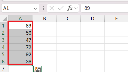
STEP 1: Identify the Data Range: Select the six cells containing the values you want to evaluate. For example from A1 to A6.

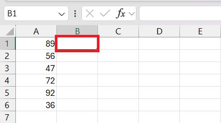
STEP 2: Select output cell: Select cell B1 where the formula will be entered.

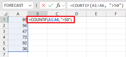
STEP 3: Use the COUNTIF Function: This function allows you to count the number of cells that meet your specified criteria within the range. For example, find numbers above 50 in the cell range A1 to A6. For this instance, enter the formula =COUNTIF(A1:A6, ">50")—this would count how many times values are above 50 in a range from cell A1 to A6.

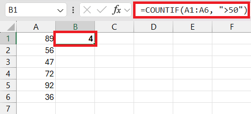
STEP 4: Check the result: Press enter and find the count. For this example, the output shall be the count of numbers that are above 50 i.e. 4.

Other formulas can be combined with the COUNTIF formula for more complex solutions.

Remember, constructing formulas requires attention to detail as one wrong character can result in errors.

 

Practical Applications of the 4 Out of 6 Calculations

Academic Grading Systems: Optimizing Student Scores

In the realm of academia, Excel’s 4 out of 6 formula can be a godsend when it comes to calculating student scores. Here’s how you might apply it:

• Individual Performance: You can determine if a student has passed by checking if they have achieved the minimum passing score in at least 4 subjects out of 6.
• Aggregate Performance: It also allows for quick assessment of class or grade-level performance.

For instance, using the formula =IF(COUNTIF(C5:H5,">=70")>=4,"Pass","Fail") enables educators to automate the pass/fail process, saving time and reducing the chances of manual errors. This way, scores can be optimized and clearly presented.

 

Business Metrics: Assessing Top Performing Segments

In the business spectrum, the “4 out of 6” calculation is quite potent for assessing top-performing segments or products. Here’s where it shines:

• Sales Analysis: Discover which products out of a selection are exceeding sales expectations.
• Performance Tracking: Identify which departments or teams have met their targets most consistently.

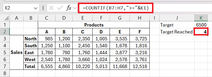
By implementing a formula like =COUNTIF(B7:H2,">="&K1), where K1 contains the target figure, managers can instantly see how often a certain sales figure or target has been hit. This dynamic application can help in strategic decision-making, ensuring focus on the most productive areas. In the example given below 4 out of 6 products reached their sales target.

 

Tips and Tricks to Enhance Your Excel Skills

Avoid Common Pitfalls: Ensuring Accurate Results

To make sure you get accurate results in Excel, keep the following in mind:

• Double-Check Parentheses: Ensure you’ve placed parentheses correctly in your formulas to avoid precedence errors.
• Decimal Conversions: Always convert percentage values to decimals in your formulas.
• Regular Audits: Periodically check your formulas and data entries for consistency and accuracy.

For example, if computing a percentage increase, the correct formula would be =((New_Value - Old_Value) / Old_Value) * 100. An error in parentheses placement could produce a completely different outcome.

Remember, even with Excel’s assistance, vigilant validation is key to maintaining the integrity of your calculations.

 

Related Shortcuts and Formulas for Efficiency

Boosting efficiency in Excel is often about knowing the right keyboard shortcuts and formulas. Here are some related tips to speed up your tasks:

Shortcuts:

• Sum: Alt + ‘+’
• Fill Down: Ctrl + D
• Insert Function: Shift + F3

Formulas:

• AutoSum: =SUM() automatically adds up numbers in a range.
• Quick Multiply: =PRODUCT() multiplies a series of numbers quickly.
• Combining Functions: Nest functions like =AVERAGE(IF()) to perform complex calculations in a single step.

Keeping a list of these efficiencies can save you time and reduce manual work.

 

FAQs

How do I automate the 4 out of 6 calculation in Excel?

To automate a “4 out of 6” calculation, use the =LARGE(range, k) function four times to find the four highest numbers and then average them, or directly use the =AVERAGE(TOP 4 of the range). This formula automatically performs the calculation each time you input or change the data.

How do I calculate 4 percent of a number in Excel?

To calculate 4 percent of a number in Excel, use the formula =number*0.04. Simply replace “number” with the value you’re calculating 4 percent from. This will give you 4% of that number instantly.

Can this formula be adapted for different scenarios, like best 3 out of 5?

Absolutely! The formula can be adapted by changing the COUNTIF range and the criteria. For the best 3 out of 5 scenario, use =IF(COUNTIF(range, ">=criterion")>=3,"Pass","Fail"), adjusting the range and criterion to fit your specific scenario.

How do you find 5% of a number in Excel?

To find 5% of a number in Excel, multiply the number by 0.05 using the formula =number*0.05, replacing “number” with the specific value you want 5% of. This will yield the desired 5% value quickly and accurately.

How do I calculate the percent remaining on an invoice log?

To calculate the percent remaining on an invoice log in Excel, subtract the amount paid from the total amount, divide by the total amount, and then multiply by 100. Formula: =((Total_Amount - Amount_Paid) / Total_Amount) * 100.