Excel Tips: How to Count and Sum by Color in Excel Effortlessly

Color-coding in Microsoft Excel isn’t merely about aesthetics; it’s a powerful aid for navigating complex datasets swiftly. By leveraging color-coded systems, you can expedite data analysis, spotting patterns and insights at a glance. In this guide, we will cover the methods on How to count and sum by color.

Key Takeaways:

• Visual Navigation: Color coding accelerates data scrutiny, turning rows of numbers into visual cues for patterns and trends.
• Conditional Formatting: Utilize Excel’s built-in tools to enhance visual appeal and speed up data analysis.
• Manual Techniques: Master the SUBTOTAL function to accurately sum by color, leveraging Excel’s filtering capabilities.
• Basic Formulas: Employ simple Excel formulas like SUMIF as a straightforward alternative to advanced methods.
• Advanced Methods: Explore VBA macros for dynamic and customizable summing by color, elevating your Excel proficiency.

 

Introduction to Color-Coded Summing in Excel

The Relevance of Color-Coding in Data Analysis

Color coding in Excel isn’t just for aesthetics; it’s a practical way to navigate through complex datasets quickly. Imagine scanning through rows of data for insights; colors can act like visual cues, significantly speeding up the process.

In data analysis, this color-coded system especially shines when you’re classifying items or highlighting key performance metrics—each hue representing a different data point or category, making patterns and trends effortlessly noticeable.

Preparing Your Excel Sheet for Summing by Color

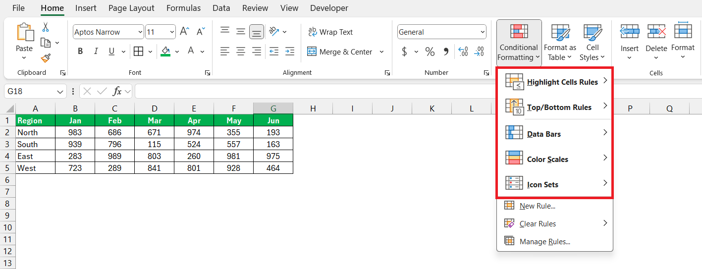
Getting your data to tell you more at just a glance with conditional formatting is quite straightforward. You start by selecting the range of cells you want to work with then head over to the ‘Home’ tab. Click ‘Conditional Formatting’ and choose from the myriad of rules available.

Whether it’s coloring cells based on their values, creating data bars, or setting up color scales, Excel’s got you covered. This not only enhances the visual appeal but can drastically reduce the time you spend looking for outliers or patterns within your dataset.

 

Manual Techniques to Sum by Color in Excel

Using the SUBTOTAL Function with Filtered Colors

Now, for summing by color, the SUBTOTAL function is a powerhouse in Excel, leaning into its ability to consider only visible rows in a filtered list.

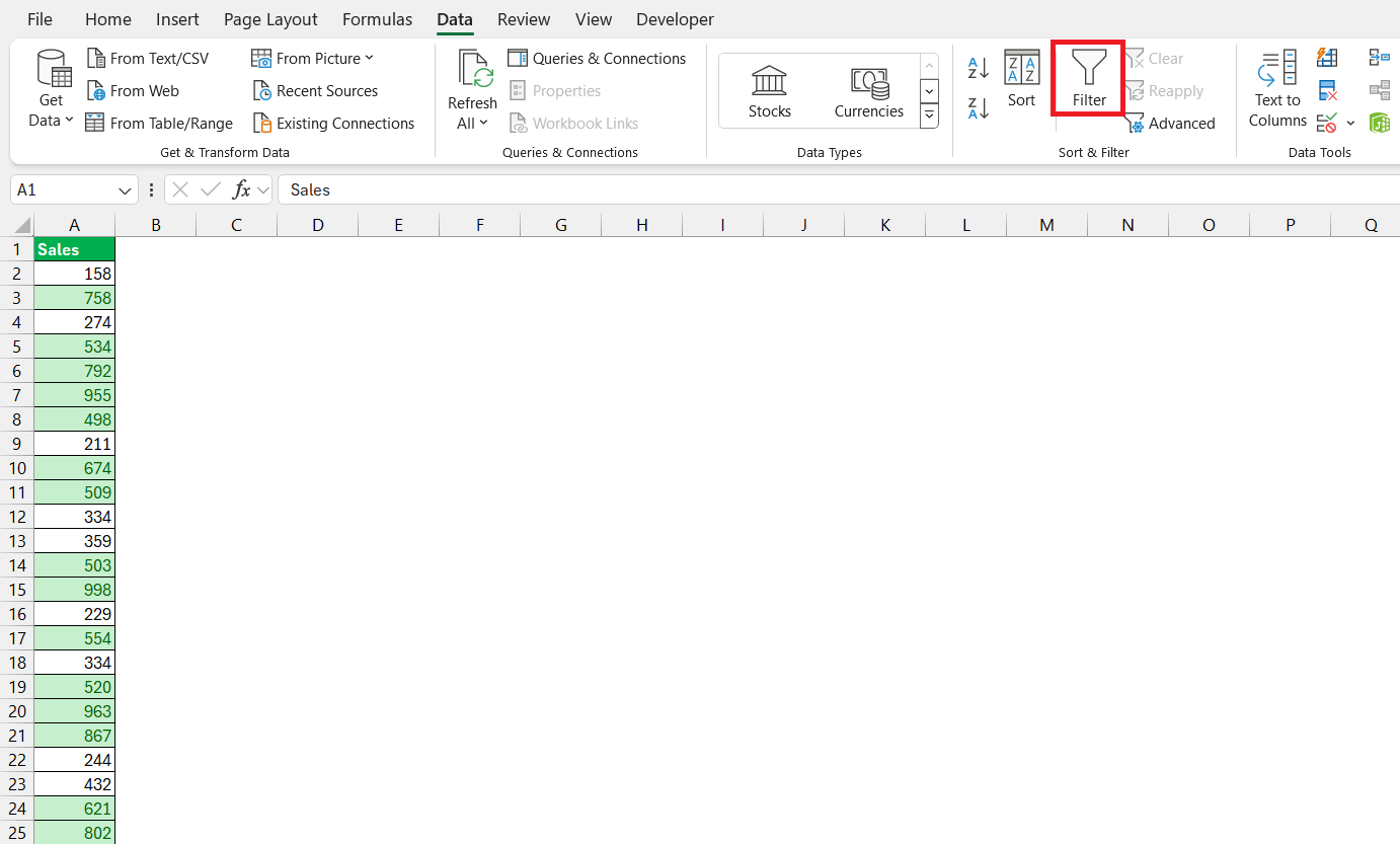
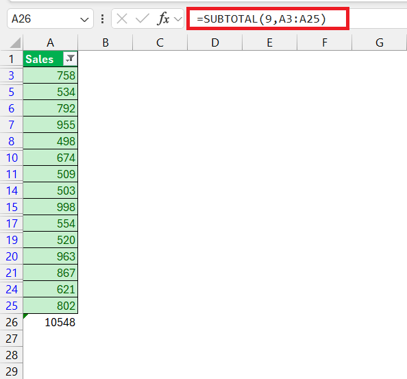
STEP 1: Start by filtering your data by the color—simply select your data, hit the ‘Data’ tab, and click ‘Filter’.

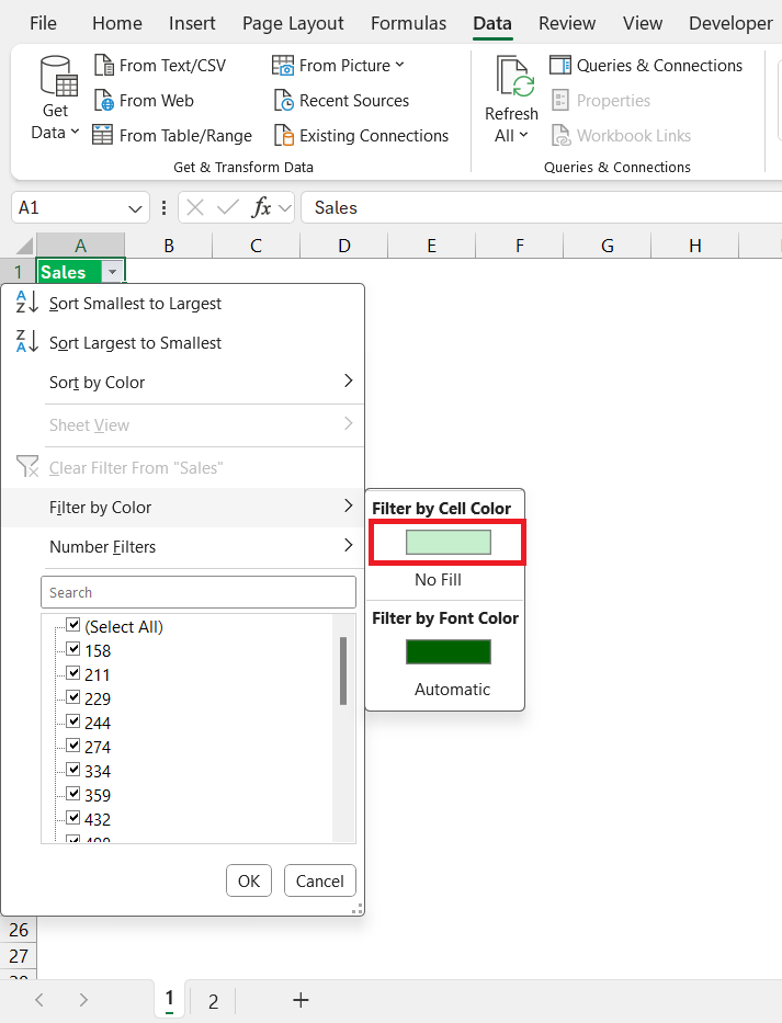
STEP 2: From there, you can choose ‘Filter by Color’ and select the color you’re interested in.

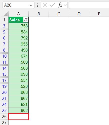
STEP 3: With your data now filtered, leave a blank row right at the bottom of the data set, this is where you’ll input your SUBTOTAL formula.

STEP 4: Input =SUBTOTAL(9, range) where ‘range’ refers to the cells you wish to sum.

This will provide you with the sum by color.

Remember, using ‘9’ as the function number ensures that you’re summing only the cells that aren’t hidden by the filter. Use 2 as a function number to ensure you get the count of the filtered cells.

 

Summing Up Cells by Color with Basic Excel Formulas

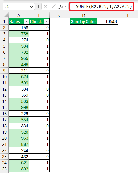
If you’re not keen on using advanced methods, basic Excel formulas can still do the trick. You’d be working on a bit of a workaround since Excel doesn’t have a built-in function for summing by color. Here’s how to approach it: use the color to define a condition, assign a value to that condition—maybe “1” for colored cells and “0” for non-colored.

Employ the SUMIF function to tally up the cells that meet your criterion.

While not directly summing by color, this method offers a simpler alternative for users less comfortable with VBA or add-ins.

 

Advanced Methods for Color-Coded Summation

Writing VBA Macros for Dynamic Summing by Color

Embrace the power of customization with VBA macros and make summing by color a breeze.

STEP 1: Press Alt + F11 to open the Visual Basic for Applications (VBA) editor.

STEP 2: Go to ‘Insert’ and choose ‘Module’ to open a blank module window.

STEP 3: Type the macro below –

Function SumByColor(CellColor As Range, SumRange As Range) As Double

Dim Sum As Double

Dim MyCell As Range

Sum = 0

‘ Check each cell in the sum range

For Each MyCell In SumRange

If MyCell.Interior.Color = CellColor.Interior.Color Then

Sum = Sum + MyCell.Value

End If

Next MyCell

SumByColor = Sum

End Function

After you have created and saved the function, you can use it directly in your Excel workbook like any other function.

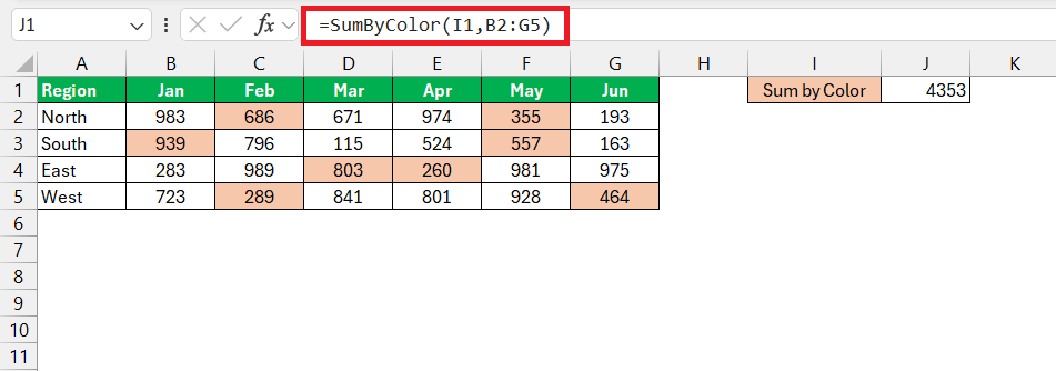
Suppose you have a cell (let’s say I1) with the color you want to sum. And you have a range of cells (B2:BG5) where some cells are colored the same as A1. You can use the function in another cell like this:

=SumByColor(I1,B2:G5)

This formula will return the sum of all cells in the range B2:G5 that have the same background color as the cell I1.

 

Tips and Best Practices for Summing by Color in Excel

Ensuring Accuracy in Color-Based Calculations

Ensuring accuracy in your color-based calculations is pivotal, as even a slight misstep can skew your data analysis. Be aware that if you’re using functions or add-ins for summing by color, they might not automatically update when cell colors change.

To guard against this, you’ll want to manually refresh your formulas or double-check the add-in settings for auto-update options. It’s also worth periodically cross-verifying your totals with a manual count, especially after making significant changes to your dataset’s color scheme.

Keeping Data Updated for Real-time Summation

To maintain the pulse of your data analysis, keeping your data updated for real-time summation is crucial. This means establishing a system where updates to cell values or colors reflect instantly in your sum totals. Make it a habit to utilize functions and tools that recalibrate automatically with each change. Dive into the settings of your Excel add-ins to ensure they’re set for automatic recalculation.

If you’re using macros, strategically place buttons to re-run them quickly. By doing so, your color-coded sums stay as dynamic as the datasets they represent, allowing you to make informed decisions on the fly.

 

FAQs on Excel Color-Coded Summing

How do I enable color-coded summing in Excel?

To enable color-coded summing in Excel, you can apply conditional formatting to your data set to highlight cells of interest. Then, use functions like SUBTOTAL to sum only visible cells after filtering by color. For more dynamic summing, you might want to write a VBA macro or use a specialized Excel add-in that provides this capability directly.

What are the limitations of using color as a criterion for summing?

The main limitation of using color as a criterion for summing in Excel is that it doesn’t inherently factor in cell color, and there’s no straightforward function for this task. Sums based on color require either manual methods, VBA scripts, or third-party add-ins. Additionally, such methods may not automatically update when cell colors change, except when using filters with the SUBTOTAL function.

Can I sum by color without writing macros?

Absolutely! You can sum by color without writing macros by using Excel’s ‘Filter by Color’ feature combined with the SUBTOTAL function to work with visible cells.

How do I total colored cells in Excel?

You can total colored cells in Excel by using its ‘Filter by Color’ feature and then applying the SUBTOTAL function to sum the visible cells in that color. Alternatively, you might opt for an add-in like Ablebits’ Ultimate Suite, which simplifies the process with its ‘Count & Sum by Color’ tool, avoiding the need for elaborate functions or manual tallying.

What is conditional formatting in Excel?

Conditional formatting in Excel is a feature that allows you to apply specific formatting to cells that meet certain criteria. You can use it to highlight, color-code, add data bars, color scales, or icon sets to your data based on its value. This dynamic tool helps in visualizing data, identifying trends, and distinguishing outliers at a glance.