How to Count Data After Filter in Excel – 3 Quick & Easy Ways

You need to tweak the data a little to see the result for the filtered data only. In this article, we will cover the following 3 methods to count data after filter in Excel –

Let us look at each of these methods.

Download the Excel Workbook below to follow along and understand How to Count Data After Filter in Microsoft Excel – download excel workbookCount-Data-after-Filter.xlsx

#1 – Use Status Bar

The easiest way to view the sum, count, or average of the filtered data is to look at the status bar. This method is handy when you want a quick count without modifying your worksheet or inserting the formula.

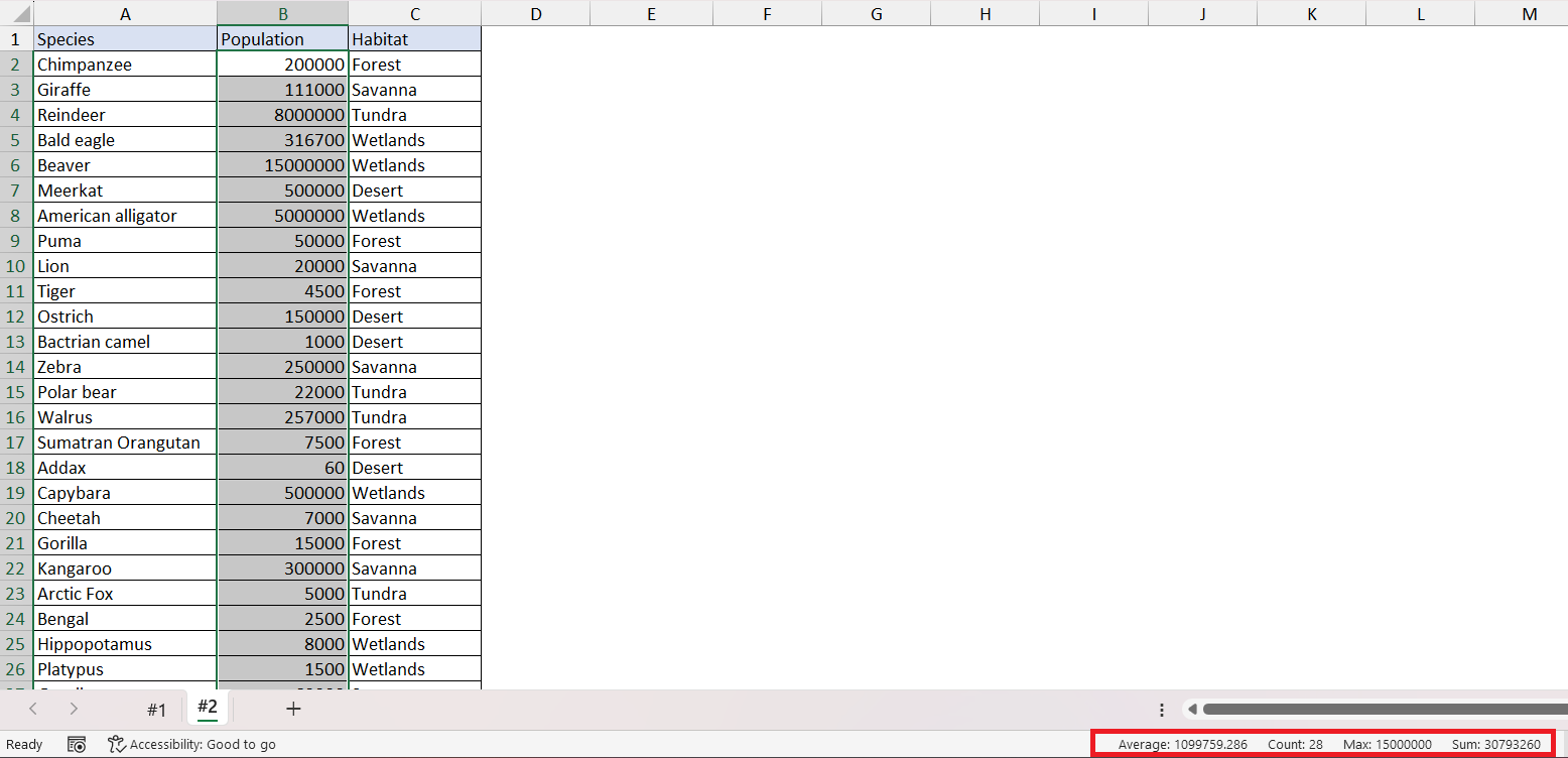
Imagine you are a biologist in charge of a dataset about various animal species in a specific region. On hand, you have data on different animals, including their species, population count, and habitat type. Let’s say you want to know the total population for a specific habitat type, such as Forest.

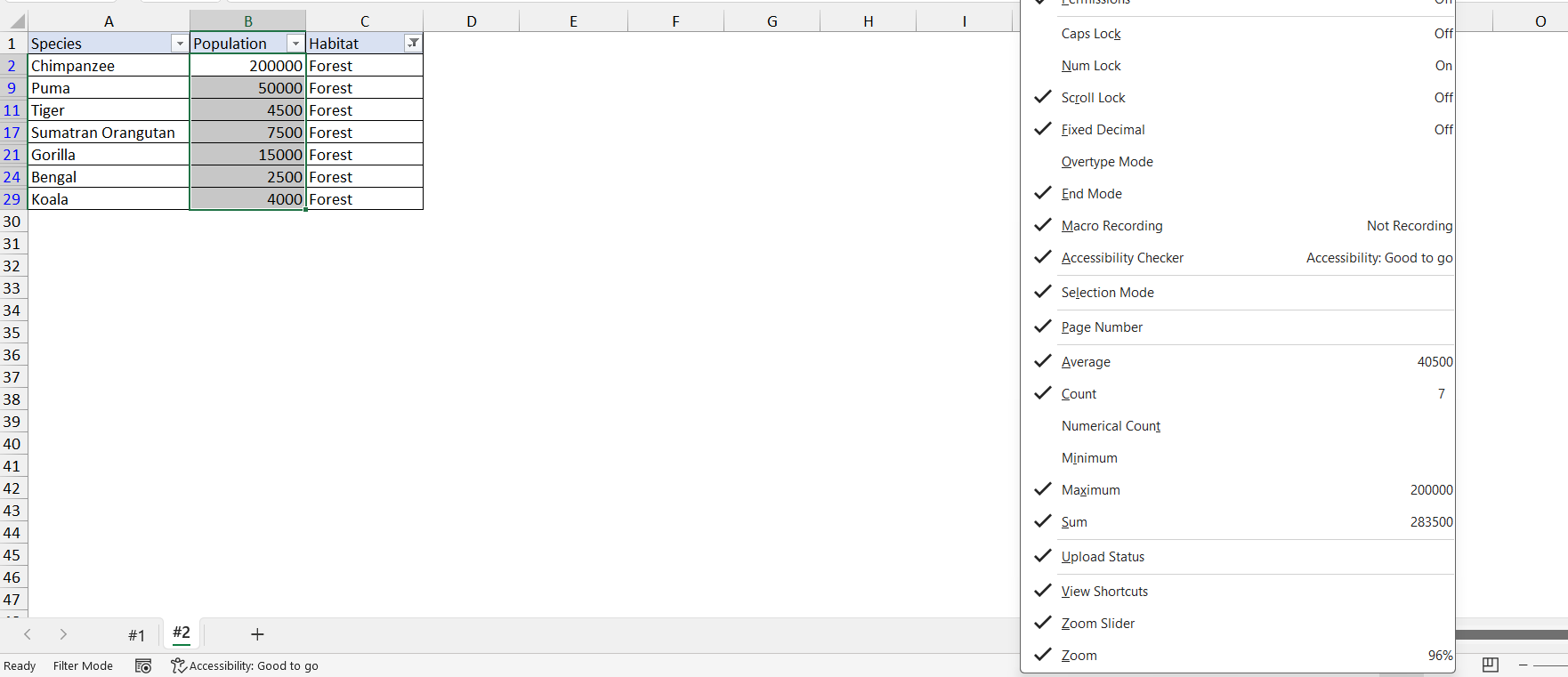
Initially, when you select the entire population column, you will that the count, sum, and average for all 28 entries are shown in the status bar.

Follow the steps below to view the calculations for filtered data only –

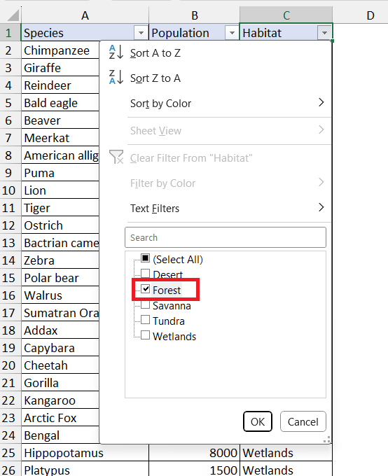
STEP 1: Filter the habitat as Forest.

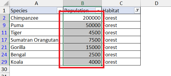
STEP 2: Highlight the entire Population column.

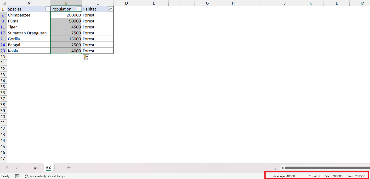
STEP 3: View the results in the status bar.

You can right-click on the status bar to see additional statistics, such as numerical count, minimum, maximum, and more.

 

#2 – SUBTOTAL Function

The SUBTOTAL function is a versatile tool that can be used to perform various calculations like sum, average, maximum, minimum, etc. One of the most useful features of this function is its ability to work on visible cells while ignoring any filtered data. The syntax of SUBTOTAL is –

=SUBTOTAL(function_num,ref1,[ref2],…)

• Function_num – It specifies the type of calculation you want to perform. Function numbers ranging from 1 to 11 include manually hidden rows, while those between 101 and 111 exclude them. Cells filtered out by Excel are always excluded from the calculation.
• Ref1 – The range or reference for which you want the subtotal.

This function is specifically designed to perform calculations on visible cells in a filtered range. Here’s how to use it –

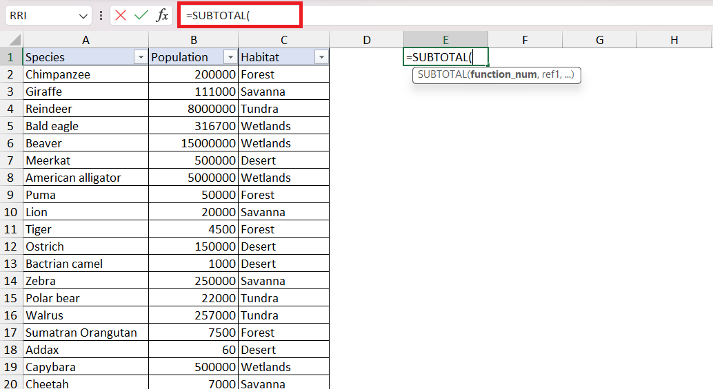
STEP 1: Enter the SUBTOTAL function.

=SUBTOTAL(

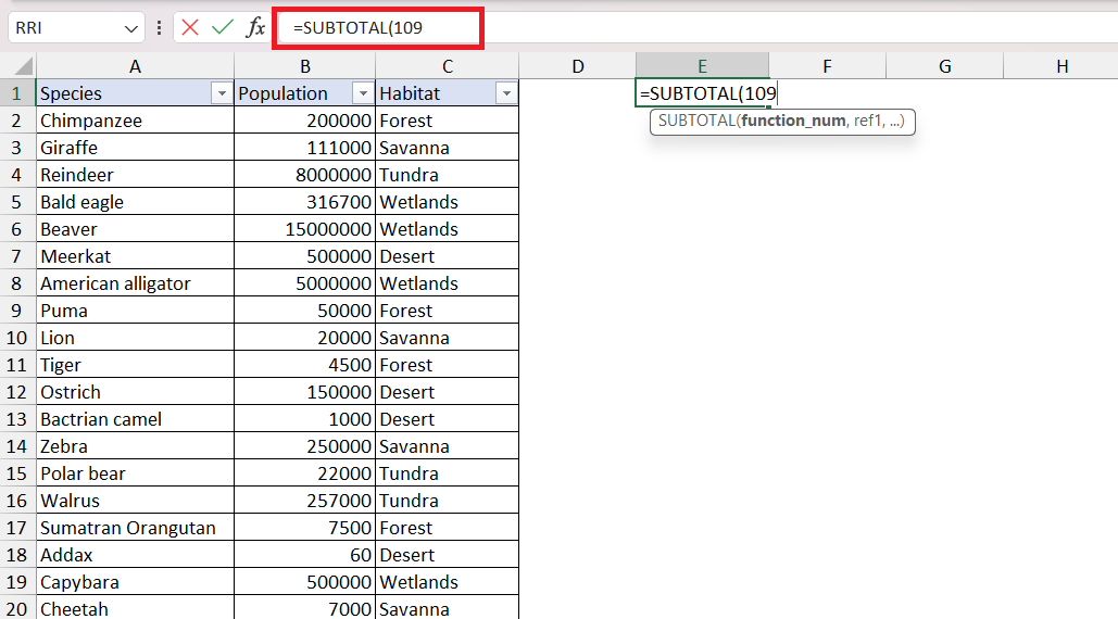
STEP 2: Enter the 1st argument i.e. function_num. Here, it is 109 as we need to use SUM to calculate the total population and exclude hidden rows.

=SUBTOTAL(109

 

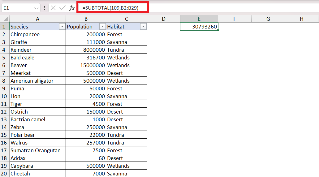
STEP 3: Enter the 2nd argument i.e. ref1. Here, it is B2:B29 as it is the range of values that contains the population.

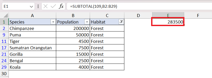
=SUBTOTAL(109,B2:B29)

By executing this formula, Excel promptly provides the total population count across all habitats.

Now, let’s delve into a practical application. Suppose we filter the data to display only the ‘forest’ habitat and observe the outcomes. It will provide the total population for forest habitat only.

 

#3 – AGGREGATE Function

The AGGREGATE function in Microsoft Excel is a versatile and powerful tool that allows you to perform various calculations on a range of data. It can also be used to count data after filter.

In the SUBTOTAL function, filtered data are always excluded. But in the AGGREGATE function, Excel provides with the option to specify your requirement. The AGGREGATE function has a flexible syntax and can be used to perform operations like SUM, AVERAGE, COUNT, MAX, MIN, and more while allowing you to ignore hidden rows and error values.

=AGGREGATE(function_num, options, ref1, [ref2], …)

• function_num – It specifies the type of calculation that you want to perform.
• options – It determines which values to ignore in the evaluation range for the function.
  • 0 or omitted – Ignore nested SUBTOTAL and AGGREGATE functions
  • 1 – Ignore hidden rows, nested SUBTOTAL and AGGREGATE functions
  • 2 – Ignore error values, nested SUBTOTAL and AGGREGATE functions
  • 3 – Ignore hidden rows, error values, nested SUBTOTAL and AGGREGATE functions
  • 4 – Ignore nothing
  • 5 – Ignore hidden rows
  • 6 – Ignore error values
  • 7 – Ignore hidden rows and error values
• ref1 – The range or reference for which you want to perform the calculation.

Let’s look at an example to understand better.

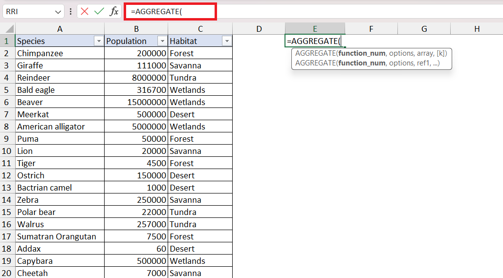
STEP 1: Enter the AGGREGATE function.

=AGGREGATE(

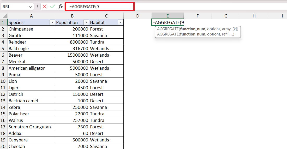
STEP 2: Enter the 1st argument i.e. function_num. Here, it is 9 as we need to use SUM to calculate the total population.

=AGGREGATE(9

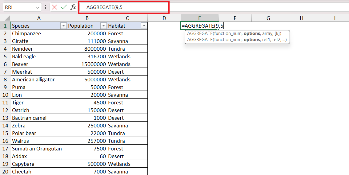
STEP 3: Enter the 2nd argument i.e. options. Here, it is 5 as we want to ignore hidden rows.

=AGGREGATE(9,5

STEP 4: Enter the 3rd argument i.e. ref1. Here, it is B2:B29 as it is the range of values that contains the population.

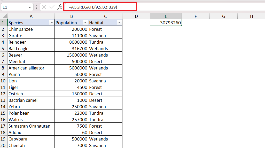
=AGGREGATE(9,5,B2:B29)

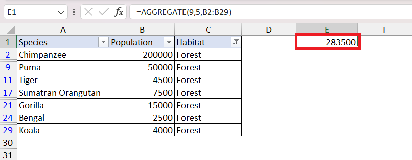
The total count for all population is displayed. Filter habitat as forest to display the count of the filtered data in the specified cell.

Further learning:

• FILTER Function in Microsoft Excel
• Change Layout of Report Filter
• Filter by Text wildcards

Click here to learn more about how to count data after filter in Excel!