Sum vs Count in Pivot Table

Ever faced the problem – The values show as a Count of rather than a Sum in a Pivot Table? This is one of the most common complaints encountered when dealing with Pivot Tables. In this article, you will be provided a detailed guide on: Summarize value as SUM, COUNT in Pivot Table, Why the Pivot Table values show as Count instead of Sum, How to fix this issue. Let’s go through each of these points one-by-one!

Summarize value as SUM, COUNT in Pivot Table

Pivot Table in Excel is one of the most powerful features within Excel that allows you to analyze more than 1 million rows of data with just a few mouse clicks.

Let’s explore the power of analyzing using a Pivot Table with the help of an example.

In the table below, you have sales data containing salesperson name, region, order date and sales amount.

Using this data, you can create a Pivot Table that tells you the number of sales achieved by each salesperson. Follow the steps below to calculate Pivot Table sum.

STEP 1: Select the Data Table.

STEP 2: Go to Insert > Pivot Table

STEP 3: In the Create PivotTable dialog box, Excel will automatically select the table for you and the default location will be New Worksheet. Press OK.

STEP 4: PivotTable panel will be created in a new worksheet.

STEP 5: You can drag and drop the Sales Person field under Row area and Sales field under the Values area.

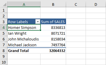
STEP 6: Below is the Pivot Table that summarizes the total sales amount by each salesperson.

By default, Pivot Table shows the summation of the sales amount. You can easily change the calculation type from Sum to one of the 11 different functions (like count, average, maximum or minimum, etc).

Right-click on the Pivot Table and select Summarize Value By > Count.

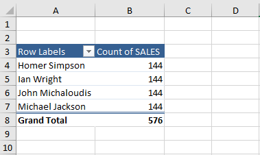
The summarization has now changed from Sum to Count Pivot Table.

Why the Pivot Table values show as Count instead of Sum

As you have seen in the previous section when you drag and drop an item in the Value field, it automatically shows the sum of the value.

But if it shows Count instead of Sum. Well, there are three reasons why this is the case:

1. There are blank cells in your values column within your data set; or

2. There are “text” cells in your values column within your data set; or

3. A Values field is Grouped within your Pivot Table.

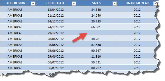
1. BLANK CELL(S):

So if you have at least one blank cell in a Values column, Excel automatically thinks that the whole column is text-based.  Pretty stupid but that’s the way it thinks.

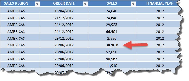
2. TEXT CELL(S):

Also if you have a cell that is formatted as Text within your Values column, then it will also cause it to Count rather than Sum.  This usually happens when you download data from your ERP or external system and it throws in numbers that are formatted as text e.g. 382821P

We get the annoying Sales Count in Pivot table below:

 

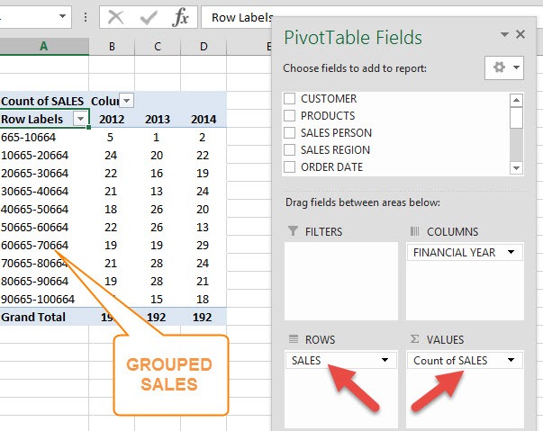
3. GROUPED VALUES:

Let’s say that you put a Values field (e.g. Sales) in the Row/Column Labels and then you Group it.

When you drop in the same Values field in the Values area, you will also get a Count of…

PivotTable basically has a set of rules which is very simple – If all the cells in the field selected contains number, the calculation type will default to SUM.

Now that you know the reason for the error, let’s learn how to fix it!

How to fix this issue

If you can clean up your data and make sure there are no cells that contain a blank, text, error, or grouped data. This will prevent the default calculation type to turn to Count in Pivot Table instead of Sum.

There are 4 ways to make sure that calculation type is set to Sum:

METHOD 1: Replace Blank with Zero

Sales column in this data table contains blank cells. Let’s use this table to create a pivot table that summarises the total sales amount by each salesperson.

When you drag and drop the Sales column to the Values area, it shows the Sales Count in Pivot Table instead of sum.

To show the summation of the sales instead of Excel Pivot Table count, you can replace the blank cells with zero.

If all the cells in the column field contains numbers, the calculation type will default to SUM.

Follow the steps below to replace blank with zero:

STEP 1: Select the entire column that contains a blank. Press Ctrl + Space Bar to select the entire column.

STEP 2: Press Ctrl + H to open the Find and Replace dialog box.

STEP 3: Delete everything in the Find what box and type 0 in Replace with box.

STEP 4: Press Replace All. This will replace all the blank cells with 0.

Now you can create a Pivot Table as all the values will contain a number!

METHOD 2: Replace Error with Zero

To replace the error message with zero, you can add an IFERROR formula.

IFERROR function is used to display custom text when a formula generates an error, and a standard result when no error is detected.

It has two arguments – value and value_if_error.

• Value – Value to be used to check error.
• Value_if_error – Value to be displayed if an error.

So if the source column contains an error, you can use the IFERROR formula to return a zero instead of the error.

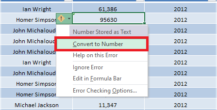
METHOD 3: Convert Text to Numbers

If a cell contains numbers but is stored as text, you will have to convert it.

To do that click on the small yellow icon on the left, and select Convert to Number.

METHOD 4: Ungroup values in the Pivot Table

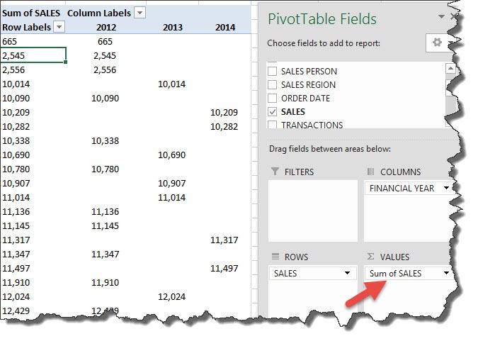
STEP 1: Right Click on the Grouped values in the Pivot Table and choose Ungroup:

STEP 2: Drag the Count of SALES out of the Values area and let go to remove it

STEP 3: Drop in the SALES field in the Values area once again

It will now show a Sum of SALES!

N.B. Sometimes you will need to locate the Pivot Table that has the Grouped values.  The SALES field may not be evident that it is Grouped, especially if it is not selected in the Row/Column labels.

You may need to drag and drop this field from the PivotTable Fields and into the Row/Column Labels area to confirm that it is Grouped.

Conclusion

In this article, you have learned how to summarize value in Pivot Table and how to make the Sum as default calculation type instead of Count when all values in the column contains numbers.

To unveil other powerful features of Excel Pivot Table, Click Here.

Further Learning:

• Clean Data Set for Pivot Table
• Prepare Data for Excel Pivot Tables
• Move and Remove Fields and Items in Excel Pivot Tables