The Ultimate Guide to Countif Not Blank in Excel

Counting non-blank cells in Microsoft Excel is a fundamental skill for anyone working with data. It allows you to focus on cells that contain meaningful information, excluding empty cells that might otherwise skew your analysis. Whether you’re managing inventory, analyzing survey results, or tracking project tasks, knowing how to accurately count non-blank cells ensures that your data insights are precise and reliable. This guide will walk you through the steps and techniques to efficiently use countif non-blank cells in Excel, optimizing your data analysis process.

Key Takeaways:

• Cell counting can be used to organize, clean, and analyze data in Excel.
• The COUNTIF function in Excel is a versatile tool that counts cells based on specific conditions, turning raw data into useful information.
• To count non-blank cells, i.e., all data except blank cells, you can use the formula =COUNTIF(range,”<>”).
• COUNTIF not blank can be used in different applications, such as finance, resource allocation, and inventory management.
• COUNTIF can be combined with other Excel functions and tools like Conditional Formatting and PivotTables to analyze data faster and more effectively.

 

Unlock the Power of Excel

The significance of cell counting in data analysis

Cell counting is useful in data analysis as it helps you in identifying trends, performing statistical analysis, and cleaning a data set. It also helps you in quantifying the amount of data and categorizing it into groups.

Overview of Countif and Its Relevance in Excel

The COUNTIF function is a key function for someone who works with a large dataset. COUNTIF is used when you want to count cells that match a single condition. This function can be used for a variety of situations:

• Count how many times the sales target was exceeded
• Count how many times a word appears in comments
• Count how many products are low in stock
• Count how many students scored above the passing score

 

Understand COUNTIF Function

COUNTIF for non-blank cells

To use the COUNTIF function for non-blank cells, you need to use this syntax: =COUNTIF(cell-range,”<>”)

Here, the cell range is the group of cells you want to check, and “<>” is a logical operator to check if the cell range is empty. This will count only the non-empty cells.

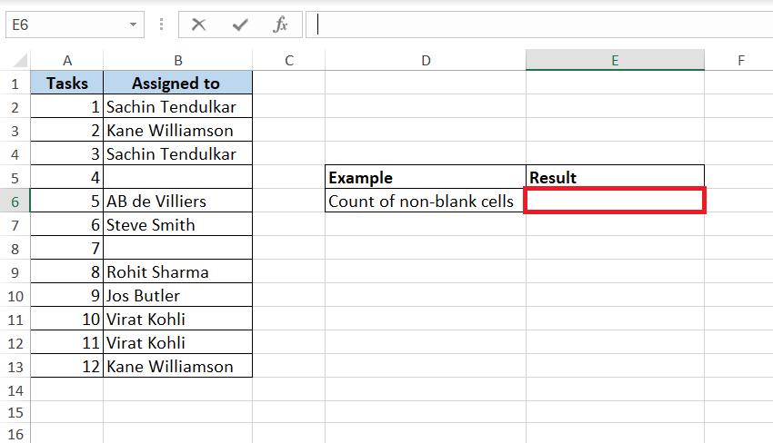
STEP 1: Select the cell where you want the result.

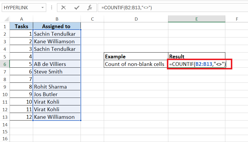
STEP 2: Enter the following formula

=COUNTIF(B2:B13,”<>”)

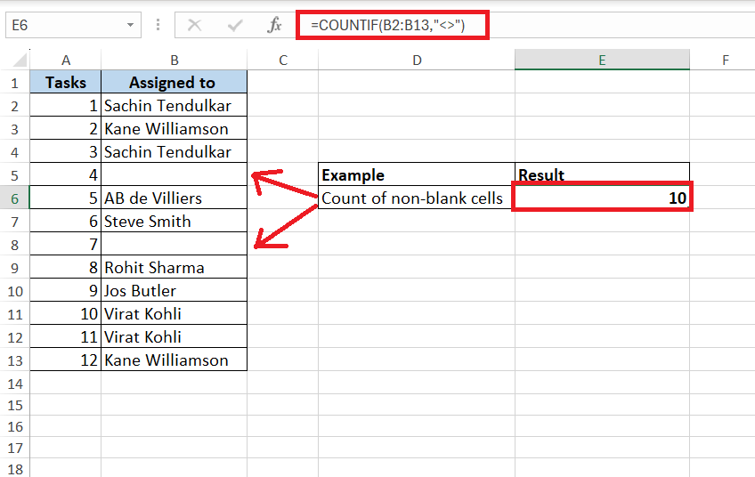
STEP 3: Press Enter. This formula will count the non-blank cells in the specified range.

Practical Uses of COUNTIF Not Blank

Excel’s COUNTIF not blank works best when you have a large and diverse dataset. Whether you’re tracking non-zero payments or checking employee records, counting non-empty cells helps you quickly see useful information.

Whether you are counting responses from a survey or checking inventory, only filled product entries matter. COUNTIF non blank acts as a radar and counts only the active data and ignores empty cells. You can use it in almost any field where you need to separate useful data from blanks every day.

Case Study: Company XYZ wants to use its resources wisely. They have a huge workforce across various projects, and they want to allocate resources more effectively.

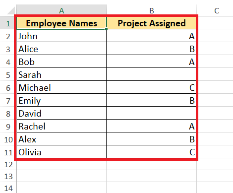
STEP 1: Enter employee names in column A and their corresponding project assignments in column B.

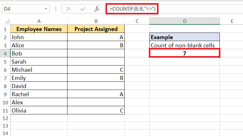
STEP 2: Use COUNTIF function in column C to count non-blank cells in column B

=COUNTIF(B:B,”<>”).

Please note the following points:

• Resource Allocation: Sort or filter the column to quickly find which employees are working on the most projects.
• Optimization: Reallocate resources from less active employees to more active employees for optimal resource utilization.
• Monitoring: Keep the data updated and check it regularly to stay efficient.

 

Diving Deeper into COUNTIF Variations

Exploring COUNTIFS for multiple criteria

COUNTIFS can be used when you want to check multiple criteria across one or more ranges. COUNTIF checks only one criterion, but COUNTIFS can check multiple criteria at once. The syntax will look like this:

=COUNTIFS(range1, criteria1, range2, criteria2,…)

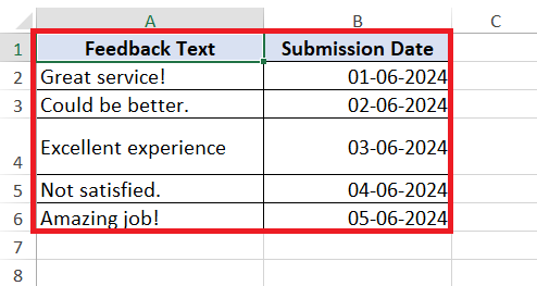
For example, imagine you have a list of customer feedback, and you want to count the number of positive responses submitted during a particular time frame. In the dataset below, customer feedback is in one column and submission date is in another column. Now, you want to count the number of positive feedback responses submitted within a certain timeframe using the COUNTIFS function.

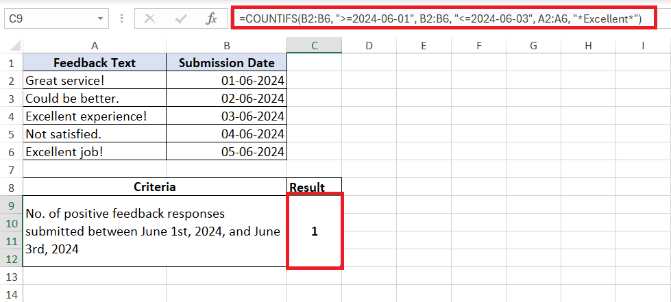
Now, let’s say you want to count the number of positive feedback responses submitted between June 1st, 2024, and June 3rd, 2024. You can use COUNTIFS to achieve this.

=COUNTIFS(B2:B6, “>=2024-06-01”, B2:B6, “<=2024-06-03”, A2:A6, “*Excellent*”)

This formula will give you the number of responses containing the word “Excellent” submitted between June 1st, 2024, and June 3rd, 2024.

Combine COUNTIF with other functions

COUNTIF becomes even more useful when combined with other Excel functions. You can use it with AVERAGE to get an average of non-blank cells, or with SUMIF to add up values that meet certain conditions. Pairing it with IF statements also lets you create custom calculations that adjust to your data. By using COUNTIF with VLOOKUP, one can find and count relevant data across different spreadsheets.

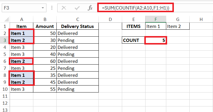
For example – COUNTIF with SUM function

 

Tips & Tricks

How to avoid common mistakes

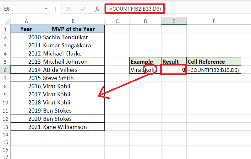
You need to be careful when using COUNTOF as even a small mistake can lead to an incorrect result. COUNTIF is case-insensitive and will give the same result for both uppercase and lowercase. You can also use wildcards for partial matches. Be mindful to check the formula carefully, use correct quotes for cell reference, and make sure the results match your expectations.

Advanced COUNTIF Techniques

Arrays and wildcards

Using wildcards and arrays along with the COUNTIF function can open a new range of possibilities. Arrays allow you to perform multiple counts simultaneously and analyze complex criteria.

Wildcards, like the asterisk (*) and question mark (?),  are extremely useful when you want to count cells that contain certain patterns or characters. They allow you to perform partial matches and go through data with varying text entries quickly and accurately.

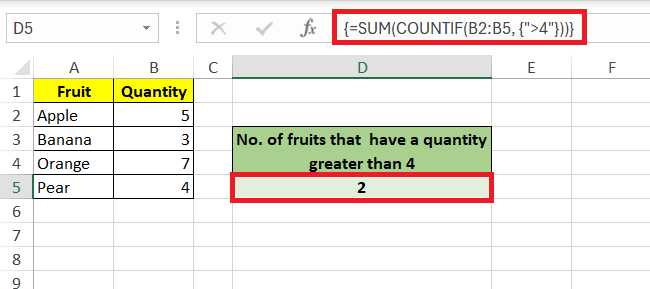
Below is an example of how to use COUNTIF with an array formula for multiple criteria:

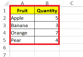
• Let’s say you want to count how many fruits have a quantity greater than 4. In an empty cell, enter the formula: =SUM(COUNTIF(B2:B5, {“>4”})). Press Ctrl+Shift+Enter to make it an array formula. The result will be the count of fruits with a quantity greater than 4.

Integrating COUNTIF with other powerful Excel tools

To truly wield COUNTIF’s potential, integrating it with other robust Excel tools can skyrocket productivity. Blend it with Conditional Formatting to visually navigate through your counts – showing cells that meet your specific criteria almost instantly.

Enrich COUNTIF with Excel’s Data Validation feature to create dropdowns that control your count criteria, making your spreadsheets interactive and error-proof. Moreover, using PivotTables in conjunction with COUNTIF simplifies the process of summarizing large datasets, giving you a comprehensive snapshot without sifting through every cell individually.

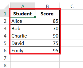
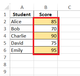
Let’s say we have a dataset of student scores in column A, and we want to highlight scores above 80.

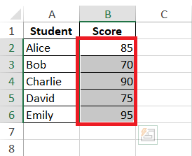
STEP 1: Select the Range: Highlight the range of cells where you want the conditional formatting to apply, e.g., cell range B2 to B6.

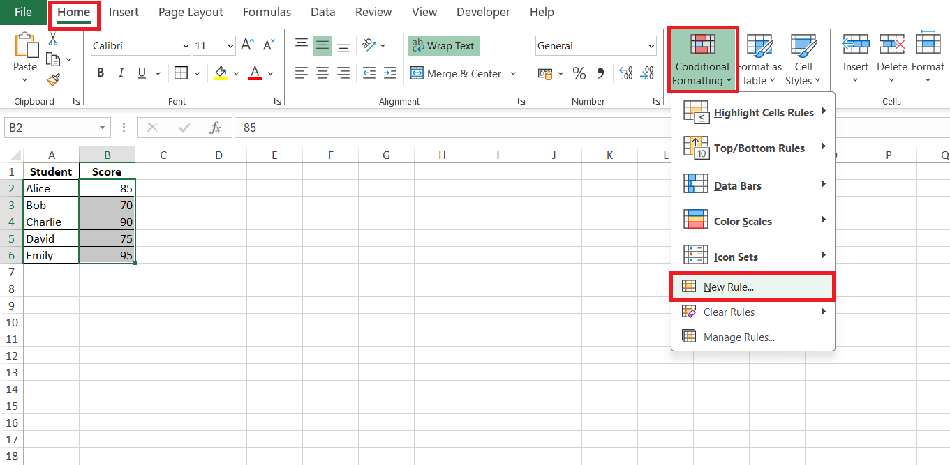
STEP 2: Apply Conditional Formatting: Go to the “Home” tab, click on “Conditional Formatting,” then choose “New Rule.”

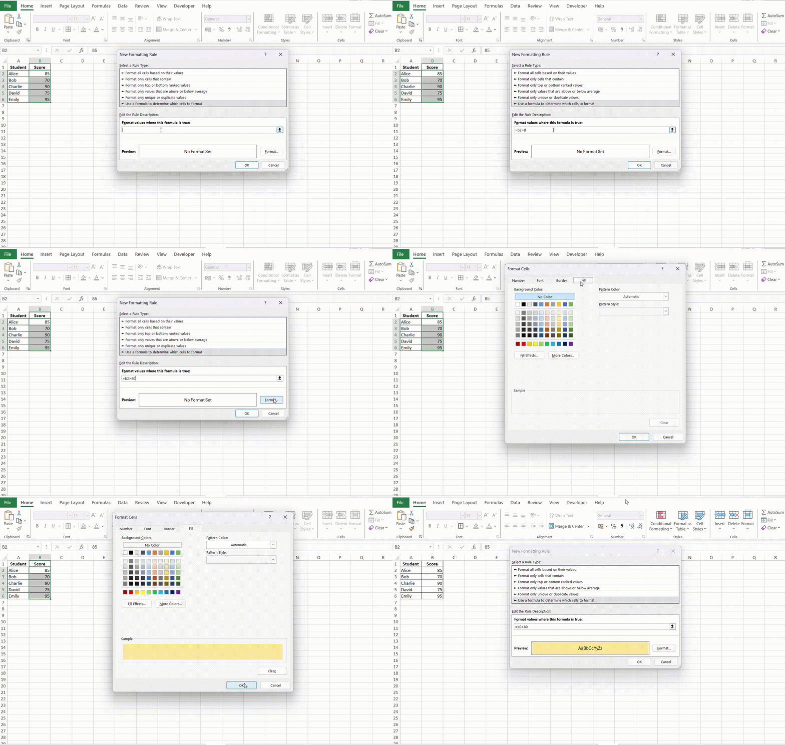
STEP 3: Set the Rule: In the New Formatting Rule dialog, select “Use a formula to determine which cells to format.” Enter the formula =A2>80 and choose your desired formatting.

STEP 4: Apply the Rule: Click “OK” to apply the rule. Now, cells with scores above 80 will be highlighted according to your chosen formatting.

 

Real-world Examples

How businesses use COUNTIF not blank for insights

Businesses use COUNTIF, not blank, as a tool to get insights from their large data set. COUNTIF not blank helps you to focus on active data only and ignore empty information.

• Retailers use COUTNIF non blank to count inventory and ignore empty shelves.
• Marketers use it to measure campaign responses and ignore unanswered calls.
• HR uses it to count complete job applications and skip unfinished ones.

Use of COUNTIF in various industries

The versatility of COUNTIF sees innovative applications across various industries. Healthcare professionals harness it to count patient cases without omitting records, bolstering patient care and service delivery. Educational institutions use COUNTIF to track student attendance, participation, and submissions. In manufacturing, precision is paramount, and COUNTIF assists in monitoring production lines, identifying bottlenecks, and maintaining steady workflow—excluding any blanks equals excluding downtime. Each industry finds its twist to COUNTIF, tailoring its strengths to their unique challenges and data practices.

 

FAQs

What is COUNTIF function?

The COUNTIF function is a formula in Excel that counts the number of cells within a specified range that meet a single given condition. This condition can range from simple numeric comparisons to text matches and even more complex patterns when combined with wildcards. COUNTIF is particularly useful for analyzing data, generating reports, and organizing spreadsheet information effectively.

What is the formula for not blank in Excel?

In Excel, to count cells that are not blank, You use the formula =COUNTIF(range,"<>"). This formula takes advantage of the “<>” operator, which means “not equal to” (also known as the “not blank” operator in this context). Replace ‘range’ with your targeted cell range for a quick count of non-empty cells in your dataset.

What is the correct syntax for the COUNTIF not blank function?

The syntax for COUNTIF not blank is =COUNTIF(range,"<>") You can replace the argument ‘range’ with the actual cell reference that you want to count. This formula will count all the cells that is not blank.

Can you count cells based on a cell’s color using the COUNTIF function?

No, the COUNTIF function cannot be used to count cells based on cell color directly as it does not evaluate cells by format, color, or other visual attributes. However, there are alternative methods, such as creating a helper column with a user-defined function or employing VBA macros, to perform color-based counting in Excel.

Why is the “@” symbol used in Excel format?

The “@” sign in the format cells represents text formatting. When you use “@” symbol in a cell’s format, Excel treats it as text. It keeps numbers, dates, and leading zeros exactly as you enter them.