Create Pivot Columns Using Power Query

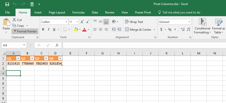
Power Query lets you perform a series of steps to transform your Excel data. One of the most common steps I do, is I want to simplify my data and aggregate them together into something like this:

Thankfully Power Query has an option that allows us to create Pivot Columns!

 

Let’s go through the steps in detail:

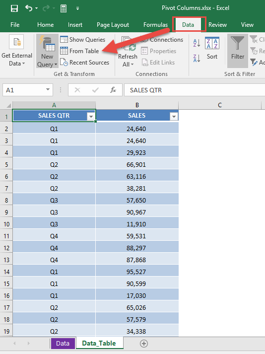
STEP 1: Our sample data consists of Sales Quarter and multiple sales values for each quarter. We want to sum them all up per quarter. Let us load our data into Power Query.

(Make sure that your data is firstly converted into an Excel Table by pressing CTRL+T and OK).

Go to Data > Get & Transform > From Table (Excel 2016) or Power Query > Excel Data > From Table (Excel 2013 & 2010)

Excel 2016:

Excel 2013 & 2010:

 

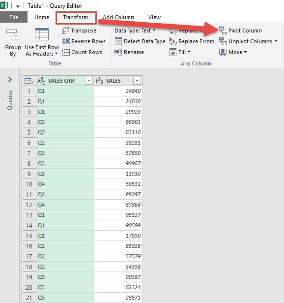
STEP 2: This will open up the Power Query Editor.

Within here you need to select Transform > Pivot Column

 

 

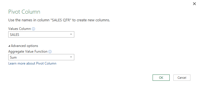
STEP 3: This brings up the Pivot Column dialogue box.

For the Values Column drop down, select the column name from our data that has the values in it…in our example it will be SALES.

Click on advanced options and this will bring up the Aggregate Value Function.  Here we select how the new cells should be combined.

As we want to show the Sales Totals for each quarter, we need to select the Sum option from the drop down box.

Click OK.

 

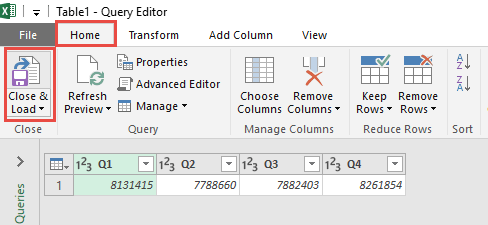
STEP 4: Now you will see your changes take place and the data has now been grouped and summed!

 

STEP 5: Click Close & Load from the Home tab and this will automatically open up a brand new worksheet in your Excel workbook with the new data.

 

You now have your new table with the total of each sales quarter.  That’s why they call it POWER QUERY!!!

 

HELPFUL RESOURCE: