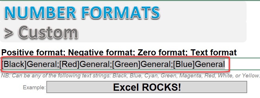
A custom number format in Excel can have up to four different sections in the following order:
Positive format; Negative format; Zero format; Text format
You can specify different format codes for each section as long as they are separated by a semicolon.
So you can display a positive number in black, a negative number in red, a zero in green and any text in blue. See the gif below to see how this can be achieved.
The following table displays the different custom codes that you can enter in the Format Cells dialogue box and how the values will appear. You can download the Excel workbook below and press CTRL+1 in each cell to see the custom format entered.
STEP 1: Copy the custom number format
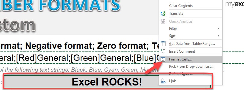
STEP 2: Press Ctrl+1 to open the Format Cells dialog. Or you can right click on the cell and select Format Cells.
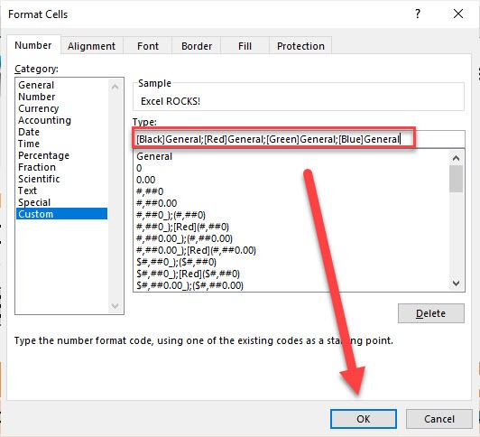
STEP 3: Choose Custom and Paste the Number Format. Then Press OK.
Try out the 4 scenarios and see them change!
- Positive – 100
- Negative – -200
- Zero – 0
- Text – Excel ROCKS!
Download workbookNumber-Formats-Custom.xlsx
| CODE | OUTPUT | HOW IT APPEARS |
| General | General format display | 123456 |
| # | Displays significant digits | 123 |
| #.00% | Displays percentage | 64.89% |
| $ – + / ( ) : | Displays this character | -$1234567890 |
| \ | Displays the next character following the \ | #1234567890 |
| “text” | Displays the text in between the quotations | 1234567890 units |
| [Color n] | Displays the color in the Excel color pallete (from 0 to 56) | 1234567890 |
| [condition value] | Custom condition eg [If it meets this condition] True Format; False Format | 1.00% |
John Michaloudis is a former accountant and finance analyst at General Electric, a Microsoft MVP since 2020, an Amazon #1 bestselling author of 4 Microsoft Excel books and teacher of Microsoft Excel & Office over at his flagship MyExcelOnline Academy Online Course.


