Customizing Excel Pivot Table Styles

There are a lot of Pivot Table Styles to choose from when you want to change the look and feel of your Pivot Table. What if even with this multitude of predefined options, you still want to make your own style? You can easily do that by customizing pivot table styles. There are a couple of ways to do this!

Key Takeaways

• Pivot Table Styles Enhance Visual Appeal – You can apply predefined styles to make Pivot Tables clearer and more professional-looking.

• Create Your Own Custom Styles – Excel allows you to design and save your own Pivot Table style, tailoring colors, fonts, and borders to match branding or personal preferences.

• Modify Specific Table Elements – You can customize different sections like header rows, column stripes, grand totals, and subtotal areas individually.

• Apply Banded Rows and Columns for Better Readability – Using banded rows/columns improves data readability by alternating row or column colors.

• Change Style Mid-Report Easily – Pivot Table styles can be changed anytime, even after data updates, without affecting the data structure.

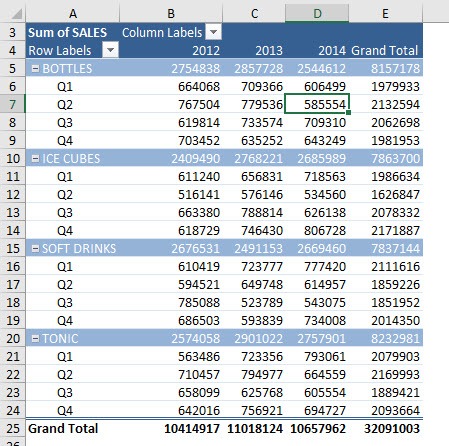
Our Current Pivot Table Setup

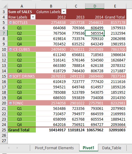
Here is our Pivot Table:

How to Customize Excel Pivot Table Styles

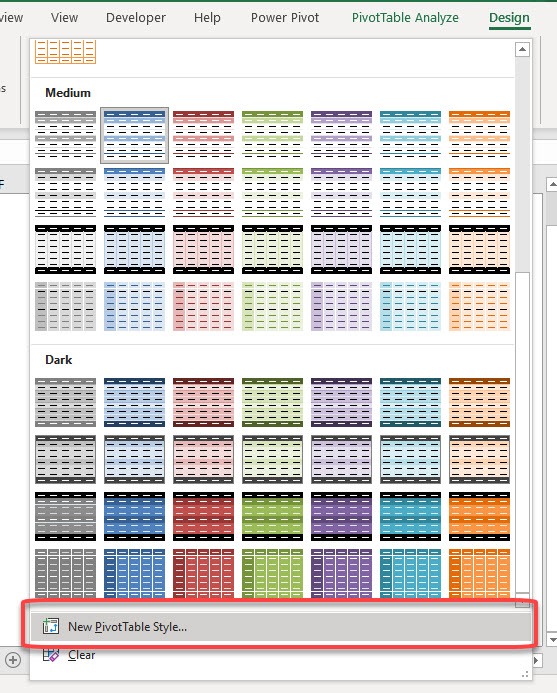
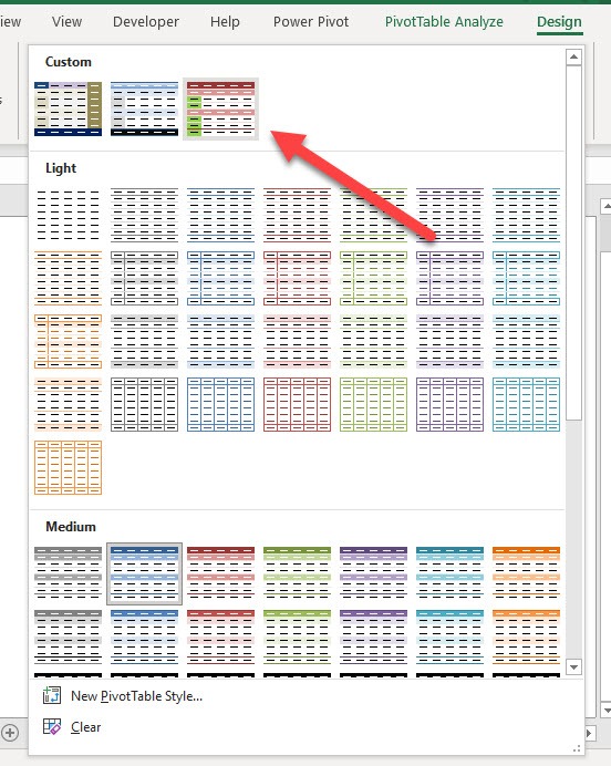
STEP 1: Go to Design > PivotTable Styles and click the down arrow to open the options

If you want to create a new custom style from scratch, select New PivotTable Style

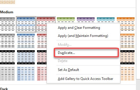
STEP 2: If you have a starting point in mind, you can right-click on any style and select Duplicate

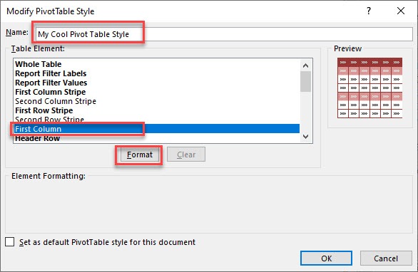
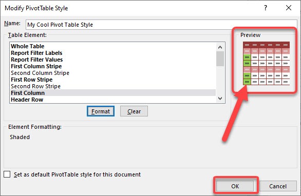
STEP 3: Change the Name into your own preference. There are a lot of elements you can format!

For our example, let us try out First Column. Select that and click Format.

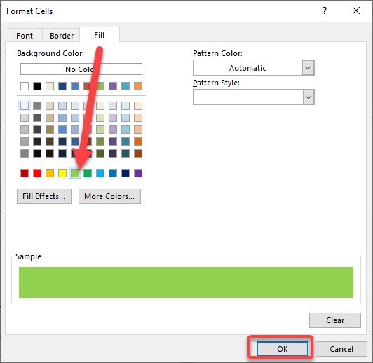
STEP 4: Try out any formatting that you want. We can try out to change the Fill color. Click OK

STEP 5: You can see a preview of how it looks like. Our first column did change its fill color! Click OK

STEP 6: The new style that we created is not applied yet automatically.

To use that, go to Design > PivotTable Styles and select the new style that we have created

And there you have it!

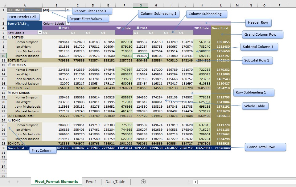
I have also created this diagram for you to immediately see the different Pivot Table Elements. Have fun creating and customising pivot table styles!

Frequently Asked Questions

Where can I find Pivot Table styles in Excel?
Go to the PivotTable Design tab → PivotTable Styles group, where you can browse through various predefined styles.

Can I create my own Pivot Table style?
Yes! In the PivotTable Design tab, click New PivotTable Style, customize the elements, and save it for future use.

Is it possible to highlight specific rows or columns in a Pivot Table?
Absolutely. Use the Banded Rows/Columns options or apply conditional formatting to highlight specific areas.

Do Pivot Table styles affect the data?
No, customizing styles only changes the appearance; the underlying data and calculations remain unaffected.

Can I apply different styles to multiple Pivot Tables in the same workbook?
Yes, each Pivot Table can have its own unique style, allowing you to differentiate tables easily within one workbook.