The #DIV/0! error is a simple error to understand. It can occur mainly when we attempt to divide two values, directly or referenced in certain cells. It is basically caused when the divisor is 0. Let’s consider different examples to examine different causes of #DIV error and learn how to get rid of DIV 0! Download the Excel Workbook below to follow along and understand better:
Key Takeaways
-
#DIV/0! Appears When Dividing by Zero – This error occurs when a formula attempts to divide a number by zero or by a blank cell.
-
Use IF or IFERROR to Prevent It – Wrap your formulas with
IForIFERRORfunctions to handle or hide the error gracefully. -
Check for Blank or Zero Denominators – Always verify the denominator cell isn’t empty or zero before performing division.
-
Use Conditional Formatting to Highlight Errors – Spot and manage cells with #DIV/0! errors visually using Excel’s formatting tools.
-
Cleaning Data Helps Avoid Errors – Ensure data is consistently filled to reduce chances of unintended divisions by zero.
Table of Contents
What is #DIV error in Excel?
Excel may return the #DIV/0! error when the:
- Number is divided by blank cell
- Number is divided by 0
If we click the exclamation warning sign beside #DIV/0! Error, excel would explain that “The formula or function used is dividing by zero or empty cells.”
How to fix #DIV Error In Excel
Example 1 – Number is divided by blank cell
The Excel DIV 0 is a common and simple error that can easily be dealt with. To correct this error, all we have to do is make sure that the cell reference provided does not belong to an empty cell.
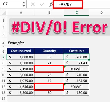
In the example below, the formula in column C is a simple dividing formula. But, cells B9 and B12 have blank cells respectively, and hence result from the division in column C returns the #DIV/0 Error.
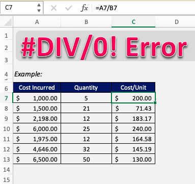
Now if we simply correct our mistakes by editing the cells in column B, the errors will disappear.
Like so!
Example 2 – Using the IF function
In most cases, the referenced cell should actually contain the value 0 or be empty. A simple solution to this will be to use an IFERROR formula and get rid of the error message.
We can design the IFERROR formula in such a way that it either returns 0 or any value as desired if the result of the original formulas occurs to be an error.
What does it do?
It returns a value that you set if a formula has an error
Formula breakdown:
=IFERROR(Value, Value if Error)
What it means:
=IFERROR(The Formula, What do you want to show if The Formula has an error?)
If you have a calculation that results in an error like, #N/A, #VALUE!, #REF!, #DIV/0!, #NUM!, #NAME?, then you can clean it up by using the IFERROR function which allows you to replace the error it with a custom text.
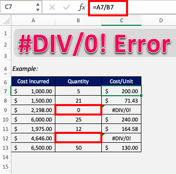
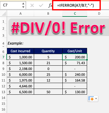
In this example, cell B9 contains 0, and cell B12 is empty. The corresponding cells C7 and C12 are thus displaying #DIV error.
Let’s wrap the division formula around the IFERROR formula and see what happens.
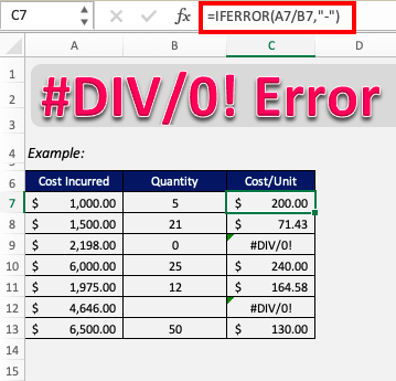
=IFERROR(A7/B7,”-“)
Here, we specified in the formula that if the value in cell C7 returns an error, it will be replaced by our custom text – hyphen (-).
Apply the same formula to the rest of the cells by dragging the lower right corner downwards.
Hence as cells B9 and B12 had blank or 0 values, the corresponding cells in column C should produce an error but IFERROR changes it to display hyphen (-).
Frequently Asked Questions
What causes the #DIV/0! error in Excel?
This error occurs when a number is divided by zero or a blank cell.
How can I hide the #DIV/0! error in a formula?
Use =IFERROR(A1/B1, "") or =IF(B1=0, "", A1/B1) to replace the error with a blank or alternative message.
Is it okay to ignore the #DIV/0! error?
It’s better to handle it using error-checking functions rather than ignoring it, especially for presentation or reporting.
Can I use formatting to manage these errors?
Yes, conditional formatting can highlight or mask cells containing #DIV/0! to improve readability.
What if I want to display a custom message instead of the error?
You can use IFERROR to show any message like =IFERROR(A1/B1, "Not Available") when the error occurs.
Conclusion
So it’s clear now that the DIV 0 error is simply caused when a number is being divided by 0 or a blank cell. If any other formula is applied on the cell displaying the #DIV/0! Error, then it will also show the same error.
Now you can easily overcome this problem and continue with smooth functioning in Excel!
John Michaloudis is a former accountant and finance analyst at General Electric, a Microsoft MVP since 2020, an Amazon #1 bestselling author of 4 Microsoft Excel books and teacher of Microsoft Excel & Office over at his flagship MyExcelOnline Academy Online Course.

