How to Create Drop Down Lists in Excel

When working with large datasets in Excel, organizing information efficiently is crucial. One of my favorite tools for streamlining data entry and ensuring consistency is the drop down list feature. In this article, I’ll walk you through the process of creating and customizing drop-down lists in Excel, which can make data management simpler and more effective.

Key Takeaways:

• Introduction to Drop Down Lists: Drop-down lists in Excel simplify data entry by providing a set of predefined choices, which helps maintain data consistency and reduce errors.
• Creating Drop Down Lists: To create a drop-down list, use the Data Validation tool to specify a range or manually enter options, ensuring users have a controlled set of choices.
• Advanced Techniques: Enhance your lists with named ranges for easier management and dynamic drop-down lists that automatically update as data changes.
• Maintaining Drop Down Lists: Regularly update and manage your drop-down lists to keep data accurate, and use error alerts to guide users in correcting invalid entries.
• Customizing User Experience: Adjust settings to allow or restrict user entries beyond the predefined options, and link multiple drop-down lists to create dependent selections.

 

Introduction to Crafting Drop-Down Lists in Excel

Understanding the Utility of Drop-Down Lists

As an avid Excel user, I’ve come to appreciate the strength of drop-down lists. These nifty tools are not just about aesthetic appeal—they fundamentally enhance the way data is handled. With a drop-down list, I can present a set of choices to users, controlling their input.

This leads to robust data integrity and a seamless user experience. Imagine handling tasks like project updates or inventory categorization. Here, the value of standardizing responses can’t be overstated; it minimizes errors and confusion.

Setting the Stage for Excel Mastery

Before we dive into the step-by-step creation of drop-down lists, it’s pivotal to establish a firm grounding in Excel proficiency. We need to lay a strong foundation built on understanding Excel’s interface, its ribbon, and where to find the necessary tools for our tasks.

Familiarizing ourselves with cell ranges, data types, and basic formulas sets us up for success. By harnessing these fundamental skills, we cultivate an environment where greater Excel mastery doesn’t just seem possible — it’s inevitable.

 

Laying the Foundation for Your Drop-Down

Selecting the Right Cells for the List

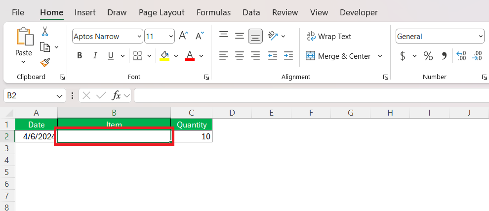
Selecting the appropriate cells for a drop-down list is a critical step that can significantly influence the usability of the data we’re managing. Begin by identifying the cells that will house the drop-down list.

For instance, if it’s an inventory sheet, this could be the column where item categories are listed. When selecting cells, consider the future expansion of the list and opt for a range that can accommodate growth.

Accessing Data Validation Tools

STEP 1: Go to the Data tab on the Excel ribbon. Click on Data Validation in the Data Tools group.

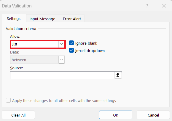
STEP 2: In the Data Validation dialog box, under the Settings tab, choose List from the Allow drop-down menu.

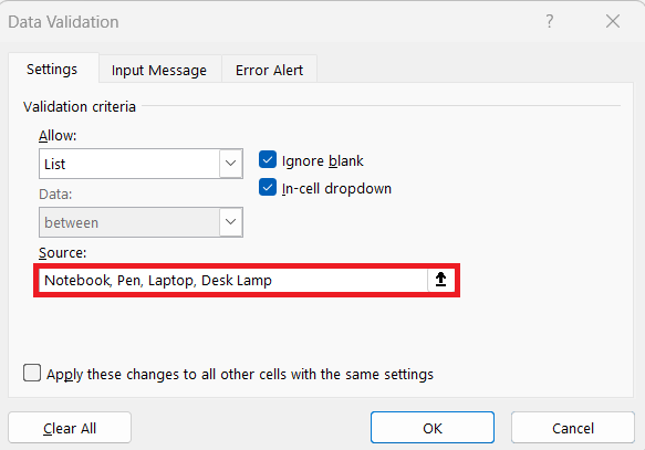
STEP 3: In the Source field, enter the items you want in the drop-down list, separated by commas (e.g., “Notebook”, “Pen”, “Laptop” and “Desk Lamp”).

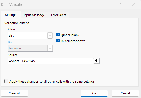
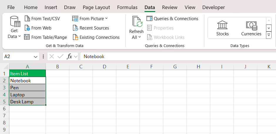
Alternatively, you can select the list of items.

STEP 4: Click OK to create the drop-down list.

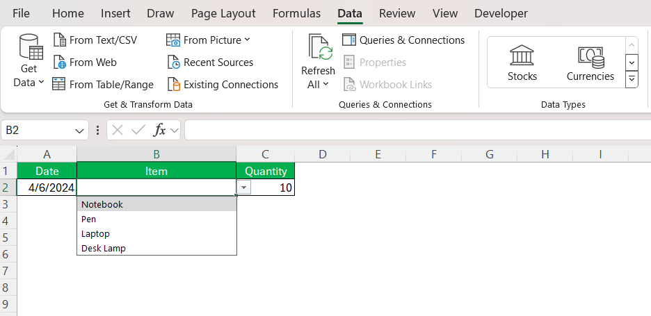
Test the drop-down by clicking on the arrow in the cell; the list of options should appear.

 

Enhancing Drop-Down Lists with Advanced Techniques

Using a Named Range

Instead of manually entering the items in the Source field, you can use a named range for your list. This method is particularly useful if you plan to reuse the list across different parts of your spreadsheet.

STEP 1: Create a list of items in a column or row.

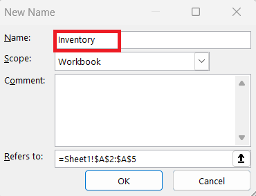
STEP 2: Highlight the list, then go to the Formulas tab and click on Define Name.

STEP 3: Give your range a name (e.g., “Inventory”).

STEP 4: In the Data Validation dialog box, enter the name you defined in the Source field, prefixed with an equal sign (e.g., =Inventory).

Dynamic Drop-Down Lists

If your list of options is likely to change, a dynamic drop-down list can automatically adjust to include new items.

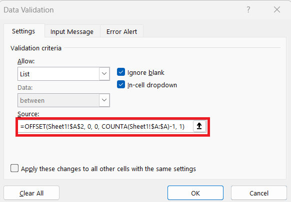
Use Excel’s OFFSET function in the Source field to create a dynamic range. For example:

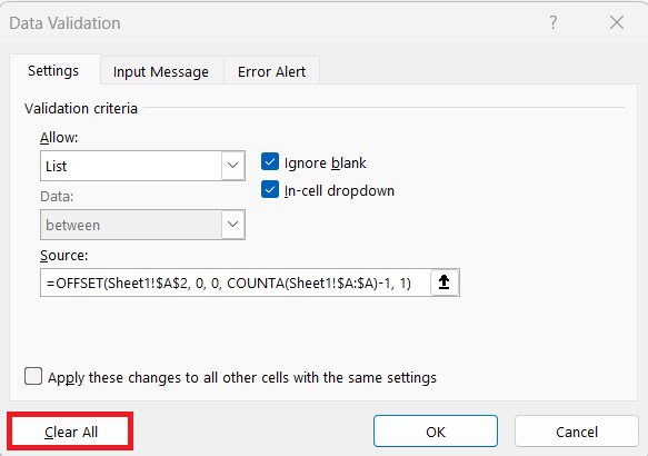
=OFFSET($A$2, 0, 0, COUNTA($A:$A)-1, 1)

This formula adjusts the range based on the number of non-empty cells in column A.

 

Best Practices for Drop-Down List Maintenance

Tips for Removing Drop down Efficiently

Here are the steps to remove a dropdown list in Excel:

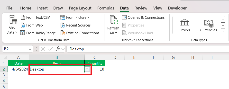
STEP 1: Click on the cell that contains the dropdown list.

STEP 2: Go to the Data tab in the Excel ribbon. Click on Data Validation in the Data Tools group.

STEP 3: In the Data Validation dialog box that appears, ensure you’re on the Settings tab. Click on the Clear All button in the bottom left corner of the dialog box. Click OK to remove the dropdown list from the selected cell(s).

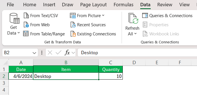
Check the cell(s) to ensure the dropdown arrow is no longer present and that the validation has been removed.

This process removes the dropdown list but retains any existing data in the cell. If you also want to clear the cell contents, you can do so by selecting the cell(s) and pressing the Delete key.

Dealing with Data Validation Errors

When encountering data validation errors, the process of resolution is as critical as creating the list itself. At times, users may attempt to enter information that does not match the pre-defined criteria in my drop-down lists, prompting Excel’s error alert system to step in. To address this effectively, I tailor error messages within Data Validation settings so that users not only become aware of the error but also receive guidance on how to correct it.

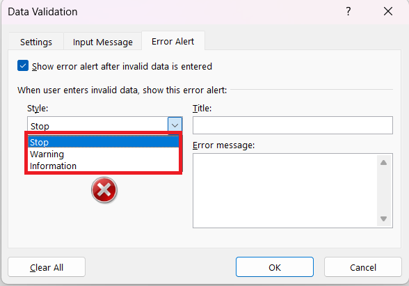
Excel provides three types of data validation error alerts to manage how users handle invalid data entries: ‘Stop’, ‘Warning’, and ‘Information.’

• The ‘Stop’ alert is the strictest option, blocking any invalid data entry entirely. Users must correct the error before they can proceed, making it ideal for critical data where only valid entries are acceptable to ensure data integrity.
• The ‘Warning’ alert offers more flexibility. It warns users when they enter invalid data but still allows them to override the warning and continue. This option is suitable when valid data is preferred but exceptions are allowed, offering a balance between enforcement and flexibility.
• The ‘Information’ alert is the least strict. It informs users that their data entry is invalid but allows the entry without restriction. This option is best used when validation criteria serve as guidelines rather than strict rules, focusing more on user awareness than enforcement.

When choosing the right alert, use ‘Stop’ for critical data, ‘Warning’ for situations requiring some flexibility, and ‘Information’ when informative guidance is sufficient

Maintaining and Updating Your Lists

Adding or Removing Items Dynamically

Keeping your Excel drop-down lists up to date can seem like a daunting task, but it doesn’t have to be. You can dynamically manage your data so that adding or removing items is a breeze, ultimately making your lists responsive to changes without the need to manually adjust their source range every time.

Here’s how you can keep your lists flexible and alert:

Adding Items:

When there’s a new entry to include, follow these steps to add it to your list dynamically:

1. Go to the cell right below the last item in your current list.
2. Type in the new item.
3. Press ‘Enter’ and voila! Your table expands and the drop-down reflects this new addition without extra steps.

Removing Items:

To remove items, the process is similarly straightforward:

1. Select the cell containing the item you wish to remove.
2. Hit the ‘Delete’ key, and the item disappears.
3. Witness your table adjusting accordingly, as does your drop-down list.

The secret to this dynamic behavior lies in formatting your list as an Excel Table. Once your source list is in this form, any changes you make automatically update the drop-down menu. It’s as simple as adding or deleting a row within the table—no need to endlessly tinker with ranges or settings.

Managing your lists dynamically not only saves time but also ensures accuracy and efficiency, especially in fast-paced environments where data changes regularly. Transform your lists into efficient tools that grow and adapt with your data!

Remember to convert your source list into a table format before attempting to utilize these dynamic features, and watch your drop-down lists become seamlessly adaptable!

Managing Dependent Drop Down Lists

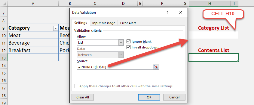
When your Excel prowess advances, managing dependent drop down lists becomes the game-changer that elevates your spreadsheets. These special drop down lists change based on the choices made in another list, paving the way for data entry that is as sophisticated as it is accurate.

Imagine having one drop down list for types of cuisine like Italian, Mexican, and Chinese, and upon selecting one, a second drop down list populates with dishes from that specific culinary style. That’s the power of dependent drop down lists.

Here’s a quick run-down on how to set up and manage these wizard-like linked lists:

1. Create a separate list in your spreadsheet for each set of dependent options. For example, one list for Italian dishes, another for Mexican, and so forth.
2. Name each list range with a unique name, ensuring these named ranges correspond to the options in the primary drop down list.
3. Use the INDIRECT function in the Data Validation settings. This function turns your selected text into a reference that Excel can use to pull up the correct named range.

To tweak your dependent drop down lists later, modify the individual named ranges – don’t forget, any changes there will reflect in the related drop down list once Excel recalculates.

Delve into Excel’s INDIRECT function to craft lists that anticipate your needs. These dependent drop downs provide clarity and user-friendliness, ensuring the data entered is precise and relevant to the context.

This is not just a feature but a centerpiece that showcases your finesse with Excel, setting your spreadsheets apart as smart, responsive, and brilliantly organized. Embrace the challenge and discover the incredible versatility that managing dependent drop down lists offers!

 

 

FAQs

How Do I Create a Yes/No Drop-Down List in Excel?

To create a Yes/No drop-down list in Excel, select the cells where you want this list to appear. Go to ‘Data’ > ‘Data Validation’, choose ‘List’ in the ‘Allow’ box, and enter “Yes, No” in the ‘Source’ field. Click ‘OK’ to finalize the list. This simple process sets up your binary list in no time.

Can I Make a Drop-Down Without Using Formulas?

Absolutely, you can create a drop-down list in Excel without formulas. Just select your cells, go to ‘Data Validation’, pick ‘List’ from the options, and enter the desired values separated by commas directly into the ‘Source’ box. Your drop-down list is ready to use, no formulas necessary!

Is There a Way to Allow Users to Enter Their Own Items on a Drop-Down List?

Yes, you can configure a drop-down list to allow users to enter items that aren’t in the pre-defined list. Go to ‘Data’ > ‘Data Validation’ and click on the ‘Error Alert’ tab. Deselect ‘Show error alert after invalid data is entered’. Users can then type their own entries, but the list will still suggest matches.

How Do I Link Multiple Drop-Down Lists?

Linking multiple drop-down lists involves creating a dependent list. Start with your primary list—say ‘Types of Cuisine’. Then create named ranges for related items—like ‘Italian’, ‘Chinese’. Use ‘Data Validation’ to create the second drop-down with a formula referencing the first list—using a function like INDIRECT. This ensures the contents of the second list depend on the first choice.

Does Excel have a drop-down option?

Yes, Excel includes a drop-down option through its data validation feature, allowing you to create a list of items for users to select from. This ensures consistent data entry and is easily accessible within the Data tab on Excel’s ribbon interface.