How to Autofit Columns and Rows in a Click in Excel

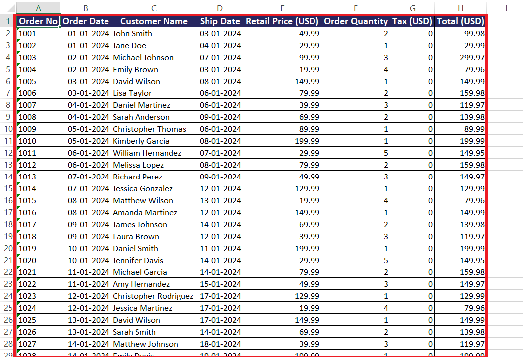
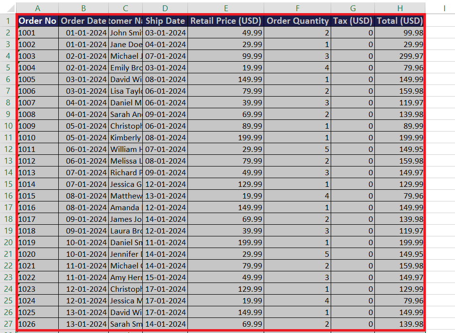
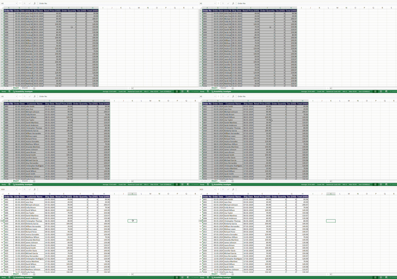
The Autofit feature in Microsoft Excel is a game-changer for managing your spreadsheets. It automatically adjusts row heights and column widths to ensure that every piece of data fits perfectly within its cell. This eliminates the hassle of manual resizing, saving you time and enhancing the professionalism of your data presentation. With Autofit, your spreadsheets become clearer and more organized, allowing for better readability and navigation.

Key Takeaways:

• Automatic Adjustments: Autofit streamlines the resizing of columns and rows, ensuring data is fully visible without manual adjustments.
• Improved Presentation: Well-sized cells enhance the professional appearance of your spreadsheets, making them easier to read and navigate.
• Keyboard Shortcuts: Using shortcuts like ALT + H + O + I for columns and ALT + H + O + A for rows can significantly speed up your workflow.
• Handling Common Issues: Autofit may struggle with merged cells or wrapped text, but simple adjustments can resolve these challenges effectively.
• Integrating into Routine: Regularly using Autofit in your workflow can improve efficiency, ensuring that your data is always presented neatly and professionally.

 

Introduction to Excel Autofit

Understanding the Autofit Feature

Imagine you’ve prepared an extensive spreadsheet, filled with data that needs to be presented clearly and professionally. Here’s where the magic of the Excel Autofit feature steps in. This handy tool automatically adjusts your row height and column width to ensure every piece of text or data fits perfectly within its respective cell.

You don’t have to manually stretch each column or row—Autofit does the work for you, saving you time and maintaining a crisp, clean look in your spreadsheets.

The Impact of Perfectly-Sized Cells on Data Presentation

An organized spreadsheet speaks volumes about the quality of your work. When your cells are perfectly sized with Autofit, your data presentation leaps to the next level of professionalism. Each value is clearly visible, without the need to squint or scroll over spilling text.

Readers can navigate through the data with ease, appreciating the readability and the uncluttered appearance of your work. Perfectly sized cells create an air of precision and attention to detail that reflects positively on you and your data-handling skills.

 

Mastering Easy Autofit Techniques

Autofit Columns and Rows with a Simple Click

With a couple of clicks, Excel’s Autofit feature quickly becomes your secret weapon for seamless data management. Here’s how you do it with just your mouse:

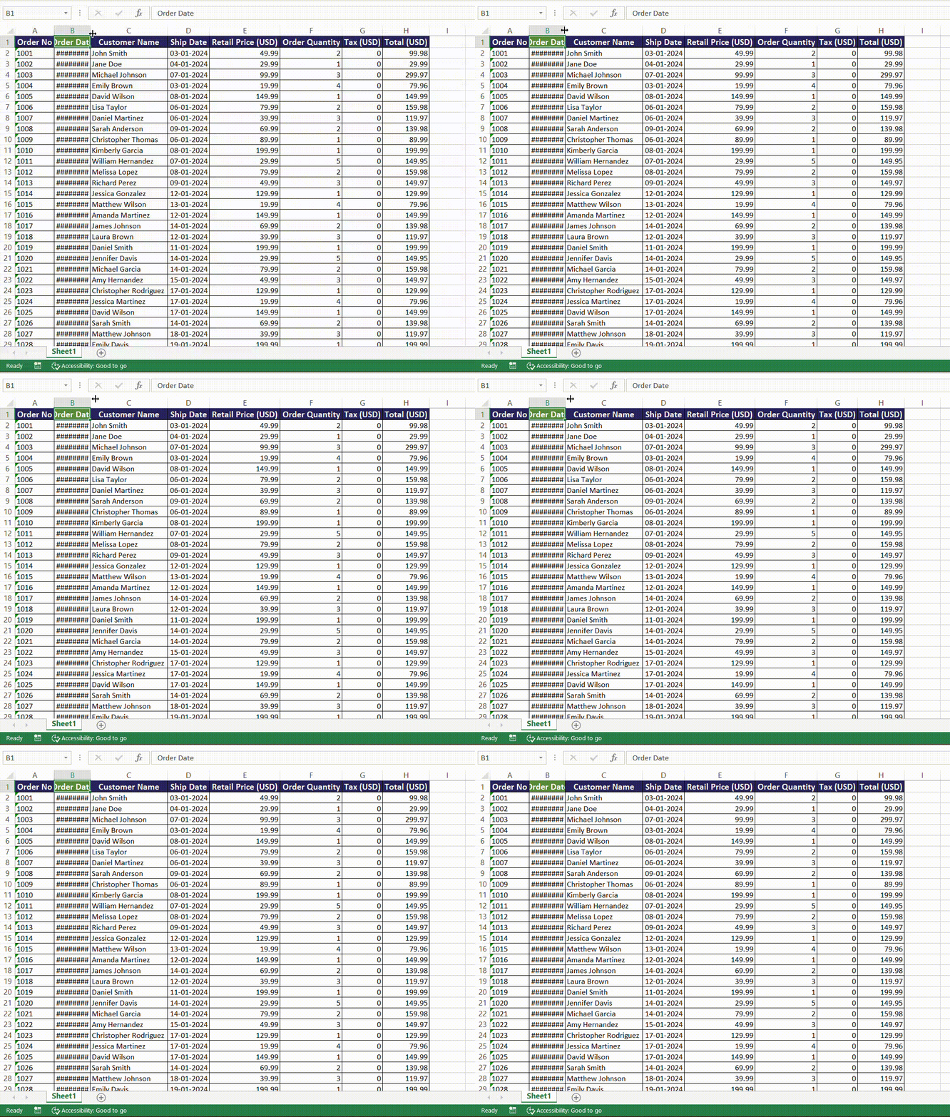
STEP 1: To Autofit a single column, hover your cursor over the right border of the column heading until it changes to a double-sided arrow.

STEP 2: Double-click, and voilà—the column adjusts to fit the widest entry perfectly.

But, what about rows? They’re just as easy:

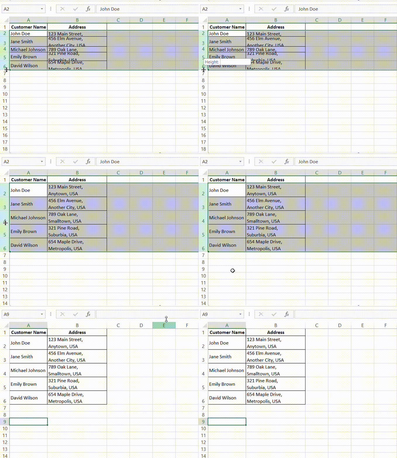
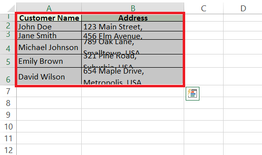
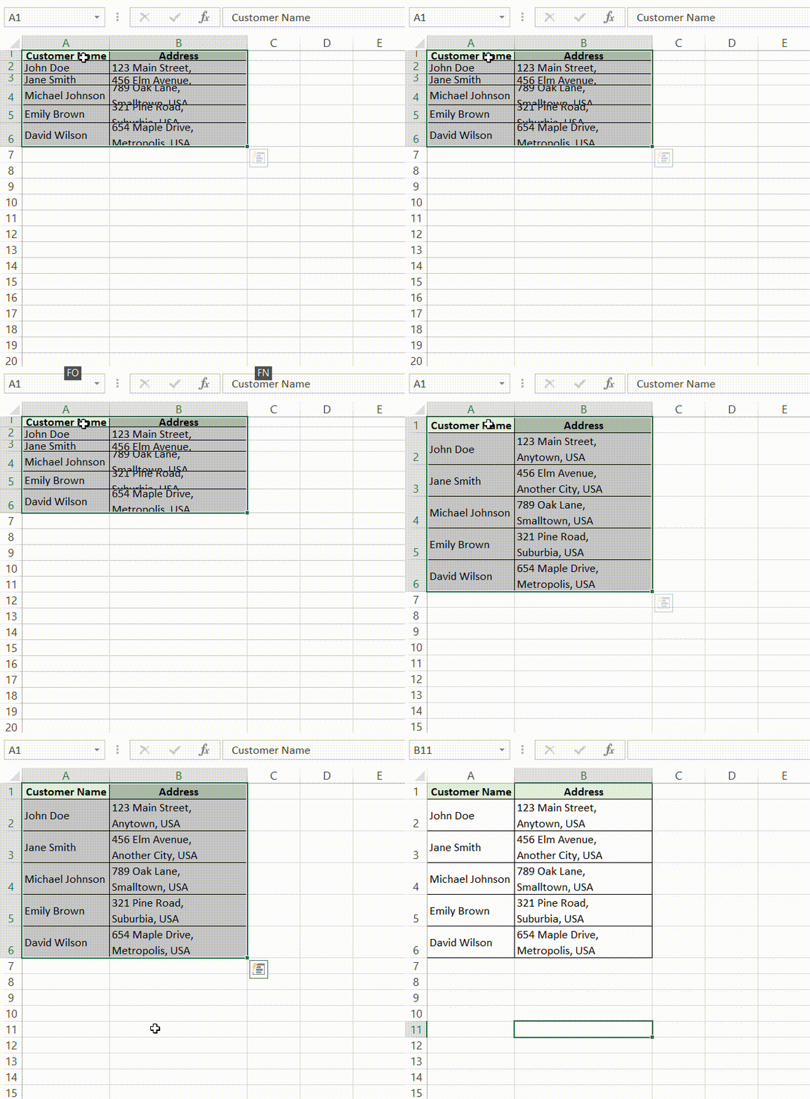
STEP 1: Select the cells where for which you want to change the row, then bring your cursor to the bottom borderline of the row header.

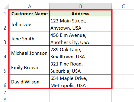
STEP 2: When you see the double-sided arrow, double-click and watch the row height adjust to fit the tallest content within.

These simple steps ensure that content is not only readable but also professionally presented. No more cut-off text or awkwardly large cells!

 

The Efficiency of Keyboard Shortcuts for Autofit

Let’s face it, efficiency is key when you’re deep in data. Keyboard shortcuts for Autofit are a game-changer for those who prefer to keep their hands on the keyboard. To quickly adjust your columns and rows to the perfect size, memorize these shortcuts:

• To Autofit column width:

STEP 1: Select your data

STEP 2: Use shortcut ALT + H + O + I. This combination swiftly resizes the column to fit the content.

• For adjusting the row height:

STEP 1: Select your data

STEP 2: Now, opt for ALT + H + O + A. Your rows will automatically expand or contract to accommodate the data.

Employing these shortcuts means you’ll spend less time adjusting your spreadsheets and more time analyzing the data that matters. It’s all about making the most of your time without sacrificing the quality of your work.

 

Navigating Common Autofit Challenges

When Excel Autofit Doesn’t Behave as Expected

Sure, Autofit is usually a reliable companion, but even the best of friends have their off days. Sometimes, you may click or tap away, expecting seamless resizing, only to be met with a stubborn column or row that just won’t comply. It seems that more often than not, wrap text is the wrench in the works, causing extra space to appear below the last line of text, or worse—overfitting that makes your data look squeezed and unreadable.

Fear not, there’s a trusted trick up your sleeve: select the whole worksheet first, then nudge any column or row border slightly. Now, give those borders a double-click, and usually, any kinks in the Autofit feature get ironed out.

These little hiccups remind you that while technology is great, it’s not infallible, and knowing how to gently persuade it back on track can save the day.

Tips for Handling Merged Cells and Text Wrapping

Merged cells and text wrapping can make your spreadsheets look smart, but they can also present unique challenges, particularly when paired with the Autofit feature. If you’ve ever tried to Autofit a column with merged cells, you might have noticed that Excel only adjusts based on the first cell in the merged set.

Here’s a lifesaver tip: to Autofit columns with merged cells, first unwrap the text. Then, find the longest piece of content that needs to fit and adjust the width of the merged cells to match it. For rows, you can often simply adjust the height manually to accommodate wrapped text.

For successful text wrapping:

STEP 1: Right-click the cell and select “Format Cells.”

STEP 2: Go to the “Alignment” tab and check “Wrap text.” Click on ‘OK’.

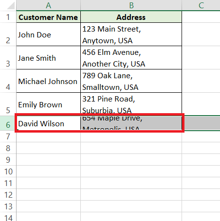
RESULT: Adjust the row height manually if needed. This lets you control how much text goes in a line and how big the cells appear, keeping everything looking top-notch.

Remember, sometimes, combining several techniques gets the best result, so don’t shy away from mixing manual adjustments with Autofit for those pesky cells.

 

Beyond Basic Autofit

Exploring Alternatives to Autofit in Excel

While Autofit is often the go-to solution, there are times when alternative methods can better suit your needs. If you’re dealing with complex datasets or design-intensive reports, it may be time to explore other avenues:

• Column Width and Row Height Setting: You can set the exact width and height by right-clicking the column or row headers, selecting ‘Column Width’ or ‘Row Height,’ and then entering your desired measurements.

• Resize to Fit Text Shortcut: Click on the border of a column or row header and drag to manually resize. Excel will show a tooltip with the measurement as you drag, allowing for precision fitting.

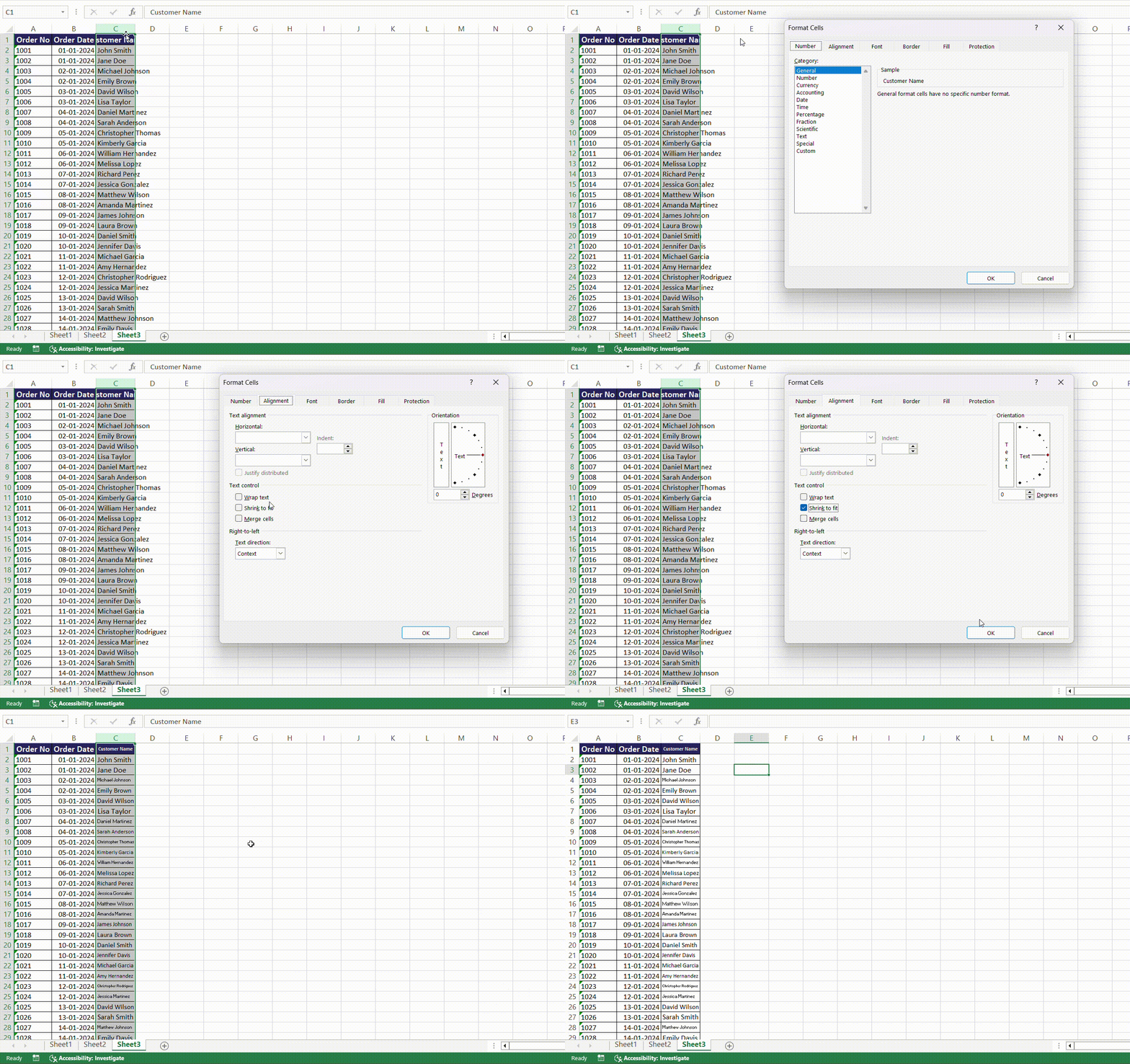
• ‘Shrink to Fit’ Option: This feature in the ‘Format Cells’ dialog box is perfect when you need to ensure the content fits into the assigned space without changing the cell’s size. The text will automatically shrink to comply.

Each alternative caters to different scenarios, and while not as quick as Autofit, they offer precision and control that Autofit can’t, ensuring your spreadsheets look exactly the way you want them to.

Setting Manual Widths and Heights for Custom Formatting

Sometimes you need a fine-tuned approach; that’s where setting manual widths and heights steps in, allowing you to have total control over your cell sizes—essential for custom formatting.

Here’s how to do it:

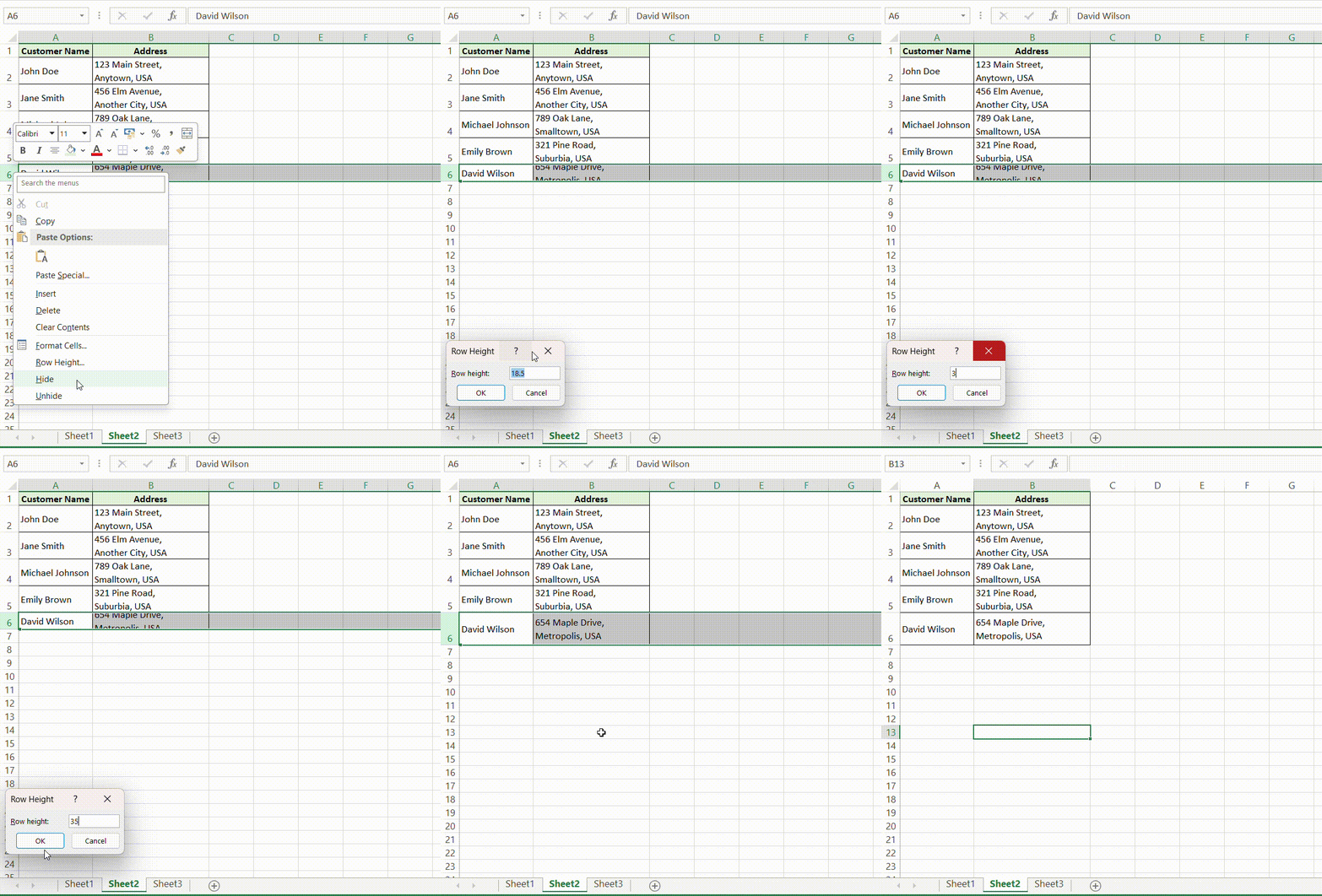
STEP 1: Select the row or column for which you want to specify the size.

STEP 2: Click the ‘Format’ button on the ribbon under the ‘Home’ tab, choose ‘Row Height’ or ‘Column Width’, then type in your desired value.

A custom format can ensure consistency across multiple sheets or make sure that your design elements, like logos or charts, have the space they need. When perfection is the goal, manual adjustment offers meticulous attention to detail that can make your spreadsheet stand out from the rest.

 

Optimizing Your Workflow

Integrating Autofit into Your Daily Excel Routine

Incorporating Autofit into your everyday Excel routine can propel your productivity, ensuring you’re working smarter, not harder. Start by getting into the habit of using it whenever you input or update data. After adding new information to a spreadsheet, a quick Autofit ensures everything is readily readable without extra effort.

For those repetitive tasks, such as weekly reporting, consider creating templates with pre-set column widths and heights that cater to your regular data input. This way, you minimize the need for constant adjustments and can trust that Autofit will work seamlessly with these prearranged settings.

Remember, consistency is key to optimizing your workflow, so let Autofit become a natural part of your Excel rhythm, and watch your efficiency soar.

Elevating Your Productivity with Additional Excel Shortcuts

When you’re ready to level up your Excel game, adding more shortcuts to your arsenal can lead to greater efficiency and productivity. Beyond Autofit, shortcuts for formatting, navigation, and data manipulation can save you clicks and time. Here’s a quick list of powerhouse shortcuts to integrate:

• Ctrl + T – Converts a range of cells to a table with quick sorting and filtering options. 2, Ctrl + Shift + L – Toggles filters on and off for your data ranges.
• Ctrl + Arrow keys – Shoots you across to the last filled cell in any direction.
• Ctrl + D – Fills down the contents of the selected cell or cells in a column.
• Alt + E, S, V – Pastes special, such as formulas, values, or formatting.

By mastering these keystrokes, you’ll navigate Excel with unprecedented speed, transforming data management from chore to a breeze.

 

FAQs

What is the AutoFit command?

Autofit is a feature in Microsoft Excel that quickly adjusts the width of a column or the height of a row to the size necessary to display the content in the cells optimally. The AutoFit command for columns is accessed by using Alt+H+O+I, and for rows, it’s Alt+H+O+A. These commands tell Excel to resize the cell dimensions automatically to fit the content, making sure that all data is visible without manual resizing.

How Can I Autofit Multiple Columns or Rows Simultaneously?

Certainly! To Autofit multiple columns or rows at the same time in Excel, just follow these steps:

• Select the columns or rows you want to Autofit by clicking and dragging across their headers.
• Double-click the boundary line between any two selected column or row headers.

This quick action will cause all the selected columns or rows to AutoFit to their largest respective entry, ensuring a neat and organized look, without any content being cut off.

What Are the Reasons for Autofit Not Working Properly in Excel?

Autofit might not work properly in Excel due to several reasons, such as the presence of merged cells, which can cause inconsistent resizing. Additionally, extra space from wrap text or content formatting can interfere with Autofit. Using older versions of Excel may also result in compatibility issues with the Autofit feature. If you encounter problems, you may need to use manual adjustments or troubleshoot the specific issues causing Autofit to malfunction.

How do you AutoFit text size in Excel?

To AutoFit text size in Excel, you use the ‘Wrap Text’ and ‘Autofit’ features combined. First, select the cells with the text you want to fit. Then:

1. Go to the ‘Home’ tab.
2. Click on ‘Wrap Text’ to enable text wrapping within the cell.
3. Adjust the column width or row height if needed by double-clicking the boundary line of the selected cell’s column or row header.

This way, Excel ensures text remains visible, adjusting the cell’s size according to its content.

How do you AutoFit cells in Excel?

Autofitting cells in Excel is a breeze. Simply select the cells, rows, or columns you want to autofit. Then, follow one of these methods:

• Double-click the border of the selected column or row header to autofit just the chosen cells.
• Use the ribbon commands under the ‘Home’ tab by clicking ‘Format’ and selecting ‘Autofit Column Width’ or ‘Autofit Row Height.’

These actions instantly resize your selections to ensure all content is visible and neatly presented.