The Ultimate Excel Column Numbering Guide – Auto-Number Tips

Have you ever needed to assign column numbers to your data in Excel? It might seem like a trivial task at first, but when working with large datasets, column numbering becomes incredibly useful. Whether it’s for referencing, sorting, or just keeping your data organized, knowing how to add column numbers efficiently can save you a lot of time. Let me walk you through some practical ways to do this in Excel.

Key Takeaways:

• Excel Column numbering can greatly enhance data organization and improve workflow efficiency.
• Methods like using the Fill Handle or functions like COLUMN() and SEQUENCE save time when working with large datasets.
• Switching to R1C1 style enables numbered headers and enhances formula referencing for advanced users.
• Excel shortcuts like F5, Ctrl + Arrow keys, and Alt + Page Up/Page Down streamline navigation across large spreadsheets.
• Auto-numbering techniques, including formulas and drag-fill methods, provide flexibility for dynamic data management.

 

Introduction to Excel Column Numbering

The Basics of Excel Spreadsheet Organization

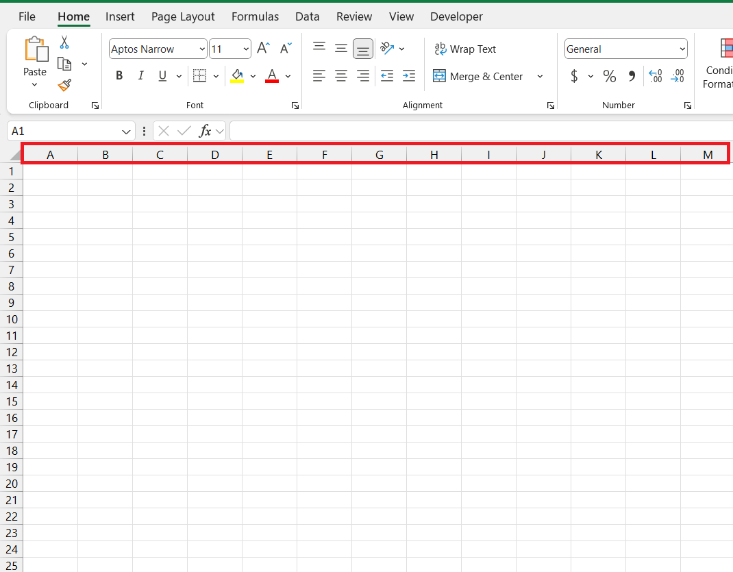
In Excel, columns are labeled alphabetically starting from A for the first column, B for the second, and so on. After column Z, the labeling continues as AA, AB, AC, and so forth. This system is known as the A1 reference style.

For example: Column 1: A, Column 26: Z, Column 27: AA, etc.

Although columns are represented by letters in the Excel interface, they also have corresponding numerical indexes that are used in formulas, coding, and other advanced features.

Column A = 1, Column Z = 26, Column AA = 27, etc.

 

Methods of Excel Column Numbering

Method 1: Manually Entering Column Numbers

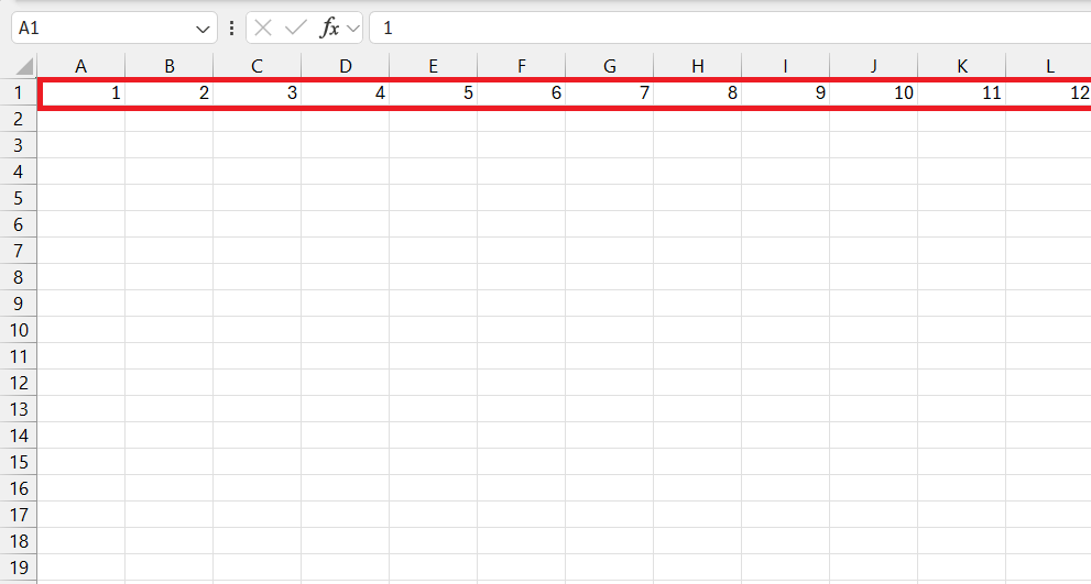
If you’re dealing with a small dataset, the easiest way to number columns is by typing the numbers manually. Here’s how I do it:

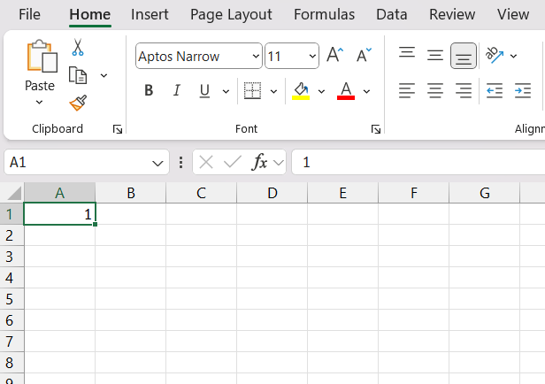
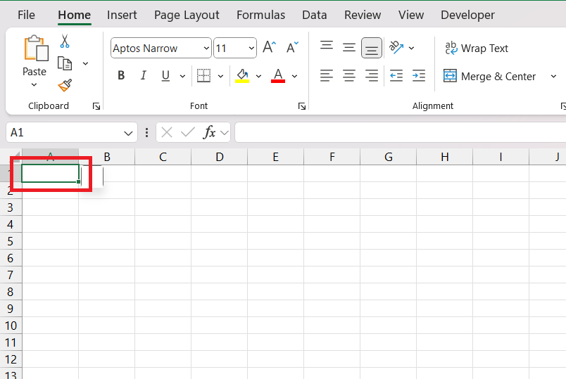
STEP 1: Click on the first cell of the row where you want the numbers to start. For example, if you want the numbers to appear in row 1, select cell A1.

STEP 2: Type 1 into the cell.

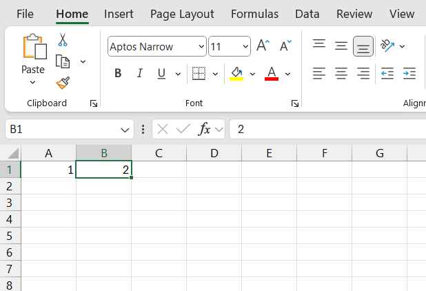
STEP 3: Move to the next cell (B1) and type 2.

STEP 4: Continue this process for as many columns as you need.

While this method is straightforward, it’s not practical for large datasets. Thankfully, Excel has built-in features to make column numbering faster and easier.

Method 2: Using the Fill Handle for Sequential Numbers

For medium-sized datasets, I often use the fill handle to quickly drag and fill sequential numbers across the columns. Here’s how:

STEP 1: Type 1 in the first cell where you want the numbering to start (e.g., A1).

STEP 2: In the next cell, type 2 (e.g., B1).

STEP 3: Select both cells to highlight them. Hover your cursor over the bottom-right corner of the selection until you see a small plus sign (“+”). Drag the fill handle across the row to extend the sequence to the desired number of columns.

This method is faster than manual entry and works well for a reasonably large number of columns.

Method 3: Using the COLUMN Function

When I’m working with very large datasets, the COLUMN function is my go-to solution. It dynamically generates column numbers based on their positions, and here’s how to use it:

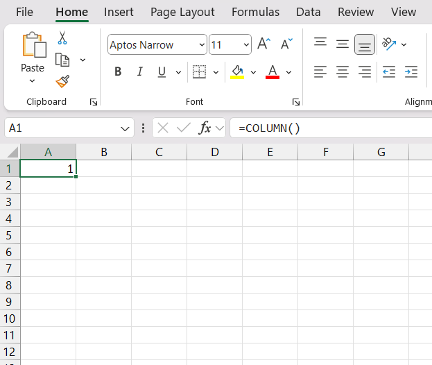
STEP 1: Select the first cell in the row where you want the column numbers to appear (e.g., A1).

STEP 2: Enter the formula =COLUMN(). Press Enter.

STEP 3: Drag the formula across the row to populate the column numbers for as many columns as needed.

The COLUMN function automatically adjusts for each column, so there’s no need to manually update anything. It’s perfect for dynamic spreadsheets where the number of columns may change.

Method 4: Using the SEQUENCE Function (Microsoft 365 Users)

If you’re using Microsoft 365 like I am, the SEQUENCE function is a powerful and efficient way to generate column numbers. Here’s how to use it:

STEP 1: Select the first cell where you want the numbers to appear (e.g., A1).

STEP 2: Enter the formula =SEQUENCE(1, COLUMNS(A:Z)), replacing A:Z with the range of columns you want to number. Press Enter.

This method automatically generates a row of sequential numbers for all columns in the specified range. It’s incredibly versatile and saves you a ton of time.

Method 5 – Switching Excel from A1 to R1C1 Style

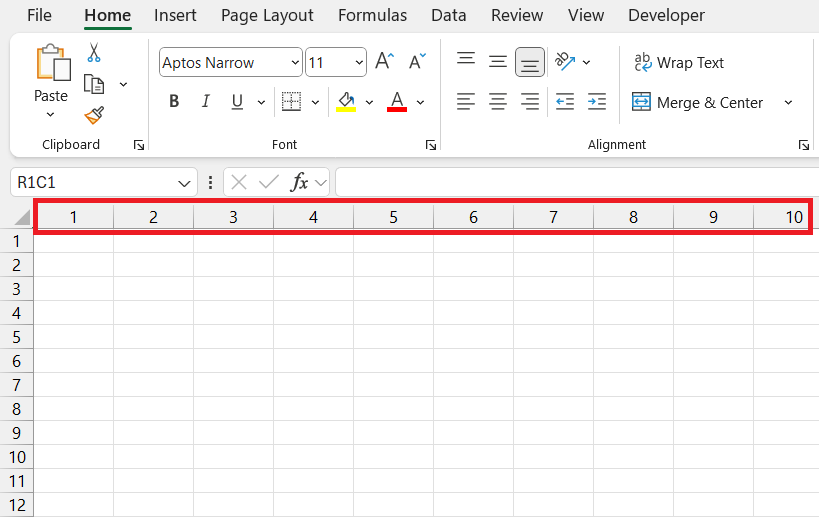
Excel allows you to use two types of reference styles for cells in formulas: A1 (default) and R1C1. The R1C1 reference style uses numerical indices for both rows and columns, making it particularly useful for advanced formula writing, automation, and understanding relative references in a systematic way.

STEP 1: Click on File.

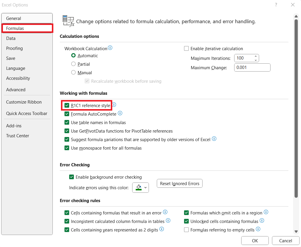
STEP 2: Select Options to open the Excel Options dialog box.

STEP 3: Navigate to Formulas in the options sidebar. Under the Working with Formulas section, check the box for R1C1 reference style.

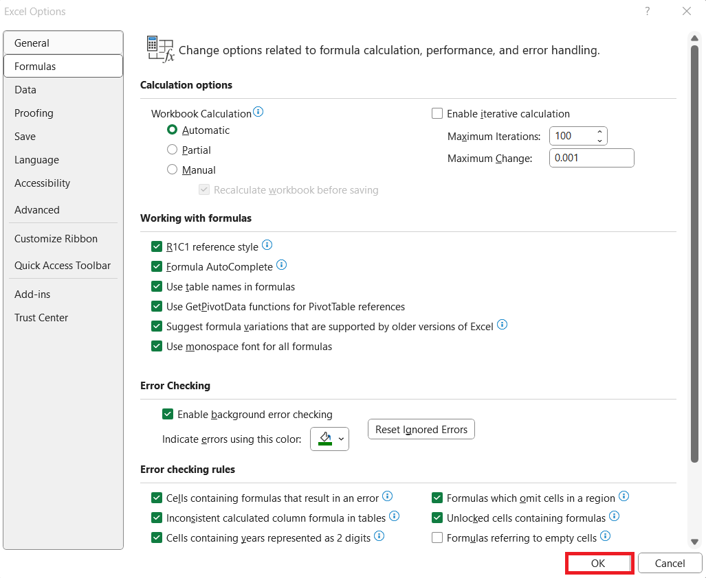
STEP 4: Click OK to apply the setting.

My column headers are now numbered, and my formulas reflect the R1C1 style.

 

Tips and Tricks for Excel Numbering Efficiency

Shortcuts for Jumping to Specific Column Lists

Now, here’s a handy trick that turns navigating Excel columns into a breeze. If you’ve ever found yourself scrolling endlessly to reach a column far across your spreadsheet, you’ll appreciate the convenience of Excel’s quick navigation shortcuts. These are the key combinations that teleport you directly to a specific column list, saving you the scroll fatigue, and boosting your productivity in the process.

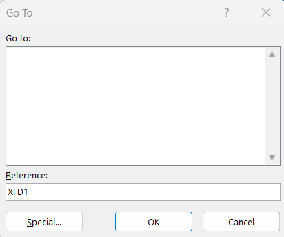
Excel’s ‘Go To’ feature (F5 key, or ‘Ctrl + G’) is akin to a GPS for your spreadsheet. Whether you’re heading towards ‘Column C’, ‘Column XFD’, or any column in between, it’s your go-to method. Simply press F5, type in the column letter followed by any row number (like ‘XFD1’), and hit enter.

Instantly, you’re exactly where you need to be—no hassle, no wasted time.

For rapid lateral movement across your columns, ‘Ctrl + Arrow key’ commands become your best friends. Holding ‘Ctrl’ while pressing the left or right arrow keys whisks you away to the furthest edge of your data in that direction. But be mindful—if you have blank cells, Excel considers those the edge, stopping your journey prematurely.

I also recommend familiarizing yourself with ‘Alt + Page Up’ and ‘Alt + Page Down’, which move your view one screen to the right or left, respectively. Consider these shortcuts the gentle nudges to the usual leap, allowing for controlled sidesteps in your spreadsheet landscape.

Each of these shortcuts offers a unique brand of efficiency. Whether you’re leaping across vast datasets or taking measured steps through your columns, mastering these can vastly cut down the time you spend in transition, giving you more time for the real work—analysis and interpretation. The key, though, is practice. Weave these shortcuts into your routine, and soon, jumping to specific column lists will be second nature.

 

FAQ: Excel Column Numbering Clarified

How do I get columns numbered in Excel?

To get columns numbered in Excel, start by selecting the first cell in the row you want to be numbered. Then, simply type =COLUMN() or 1 if you’re in the first column and press Enter. Lastly, drag the Fill Handle across the row to auto-fill the remaining cells with consecutive numbers reflecting each column’s number. If new columns are added or removed later, Excel will automatically adjust the numbers.

How Can I Extend Column Numbering Beyond ‘Z’?

To extend column numbering beyond ‘Z’ in Excel, you can continue the alphabet sequence by using double letters starting with ‘AA’. Excel does this automatically when new columns are added past ‘Z’. For an extensive grid, Excel uses triple letters after ‘ZZ’ up to ‘XFD’, giving you a total of 16,384 columns to work with for comprehensive data analysis and organization.

How do I turn off R1C1 in Excel?

To turn off the R1C1 reference style in Excel and revert to the default A1 style, follow these steps: Click on the ‘File’ tab, then choose ‘Options’. In the ‘Excel Options’ dialog box, select ‘Formulas’. Under the ‘Working with formulas’ section, uncheck the ‘R1C1 reference style’ box. Click ‘OK’ to apply the changes, and Excel will display columns with letters and rows with numbers.

What Are Some Efficient Ways to Auto-Number Rows in Excel?

Efficient ways to auto-number rows in Excel include using the Fill Handle to drag a starting number down a column, creating a simple formula like =ROW()-1, that automatically updates with row additions or deletions, or using =OFFSET() for more complex numbering. Both methods maintain a sequential order while accommodating changes in your data set, ensuring continuous numbering without manual updates.

How do I auto-number a column in Excel?

To auto-number a column in Excel, enter 1 in the first cell of your column. Then, move your cursor to the corner of this cell until it becomes a Fill Handle (a small plus sign), and drag it down to fill the cells below with consecutive numbers. For a dynamic method, use a formula like =ROW()-1 in the first cell, then drag the Fill Handle down. This will automatically adjust the numbers if rows are added or deleted.