Excel Compare Two Cells – Step by Step Guide

If you’ve ever worked on a large Excel spreadsheet, you know how useful it can be to compare data across different cells. Whether it’s checking if two values are identical or seeing if one number is greater than another, Excel provides multiple ways to compare two cells.

In this guide, I’ll walk you through some of the simplest yet most effective methods on Excel Compare two cells.

Key Takeaways:

• Comparing two cells in Excel is crucial for data accuracy and integrity.
• Use the equals operator or EXACT function for quick comparisons, depending on case sensitivity.
• Conditional Formatting visually highlights differences or matches in large datasets.
• The IF function allows for complex comparisons and customized responses.
• Excel’s data visualization tools help uncover patterns and anomalies in comparative analyses.

 

Introduction to Excel Cell Comparison

The Importance of Accurate Cell Comparisons in Data Analysis

As I dive into the world of Excel, it becomes clear that accuracy in cell comparison is the cornerstone of robust data analysis. It’s paramount for data analysts like myself to ensure data integrity, as this influences business insights, forecasts, and strategic decisions.

The meticulous process of comparing cells can unearth discrepancies that might otherwise compromise the validity of an entire dataset.

 

Fundamental Techniques of Excel Compare Two Cells

Using the Equals Operator for Direct Comparison

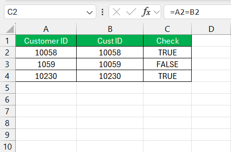
When I need to compare two cells quickly, the equals operator becomes my go-to tool. It’s straightforward: by entering =A2=B2 into a cell, Excel evaluates whether the contents of cell A2 and B2 are exactly the same.

A “TRUE” signifies a match; a “FALSE” means they differ. This direct comparison is perfect when reviewing lists or when my objective is a simple binary result indicating data uniformity or discrepancy.

The EXACT Function: Ensuring Case-Sensitive Matches

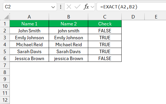
I often encounter situations where case sensitivity in data is crucial, and that’s when I turn to the EXACT function. This function is a lifesaver because it hones in on the fine details, distinguishing between ‘Apple’ and ‘apple’.

For example, by entering =EXACT(A2,B2) in a Results column, I can ascertain if two text values match in every aspect, including their case. This function returns “TRUE” only if both cells are identical in every way and “FALSE” otherwise.

It’s immensely helpful when the distinction between uppercase and lowercase characters carries meaning or impacts data classification.

• Helpful for distinguishing between textual data where case-sensitivity matters.
• Ensures precise matching, useful for password verifications or when merging case-sensitive identifiers.

 

Leverage IF Conditions for Complex Comparisons

In my toolbelt of Excel functions, the IF statement is a versatile tool that allows me to perform complex comparisons. It’s particularly powerful when the comparison criteria involve more than a simple yes or no.

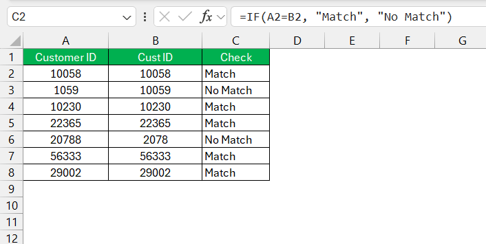
By using IF conditions, I can specify different outcomes based on whether the comparison is true or false. For instance, =IF(A2=B2, "Match", "No Match") will display “Match” if the cells are equivalent or “No Match” if they’re not.

This allows for clear, immediate interpretations of data relationships and conditions, all within a cell’s grim confines.

• Great for applying specific actions or labels to data based on the results of the comparison.
• Offers the flexibility to set up customized responses that go beyond typical true or false outcomes.

 

Visual Aids for Cell Comparison

Conditional Formatting to Highlight Differences or Matches

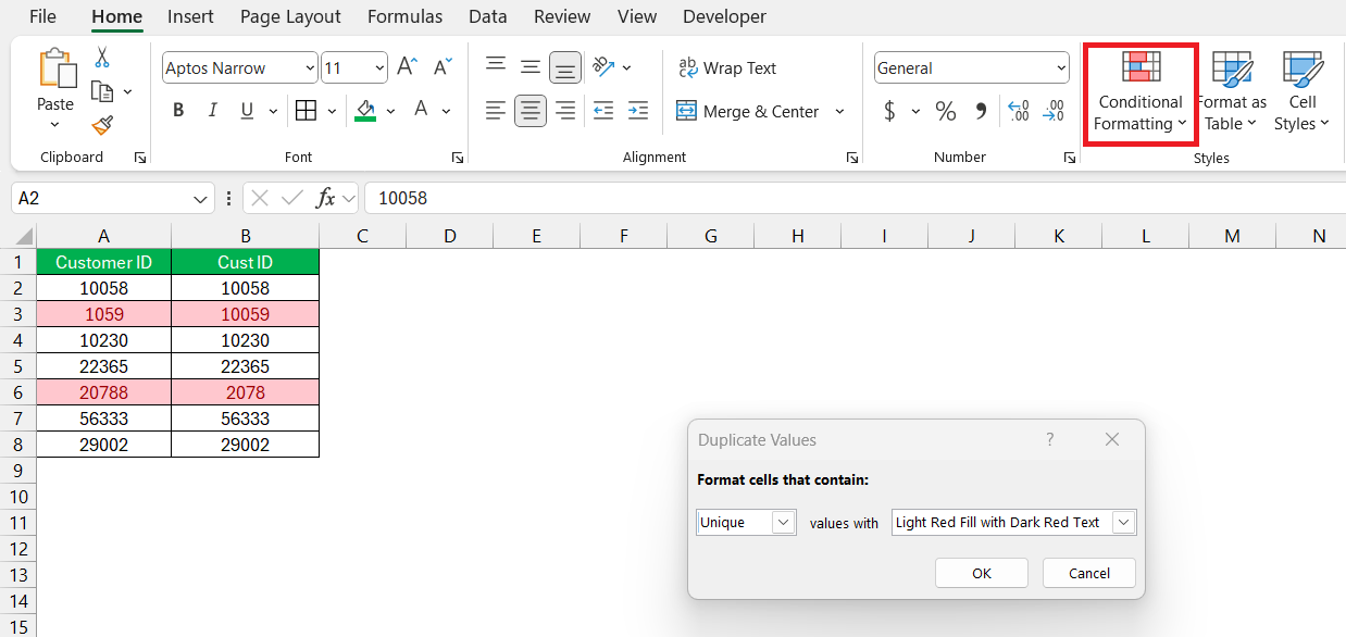
I’ve found conditional formatting invaluable for its ability to instantly highlight differences or matches in Excel. By visualizing data distinctions with color coding or other formats, we can rapidly spot what we’re looking for without wading through rows of data.

To use it, I simply select the range I want to analyze, choose ‘Conditional Formatting’ from the ‘Home’ tab, and set my criteria—like highlighting duplicate or unique values.

It’s a real game-changer, enabling a clear focus on data anomalies or confirmations at a glance.

• Streamlines identifying discrepancies or confirmations within large datasets.
• Offers flexible formatting options to customize how differences or matches are presented visually.

 

Data Visualization Tools to Identify Patterns and Anomalies

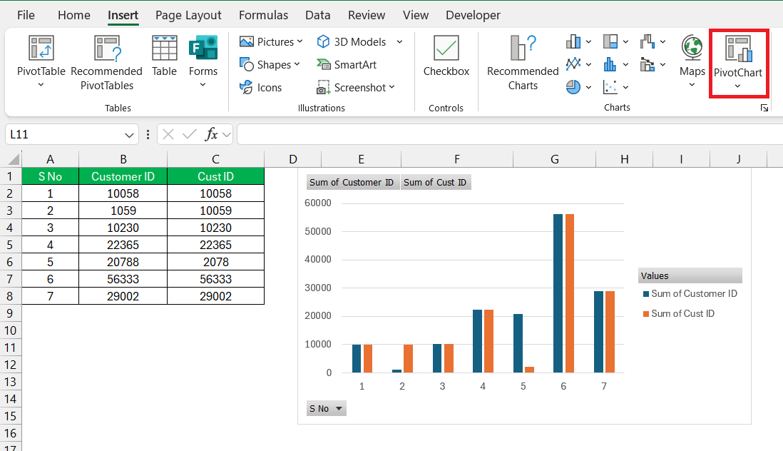
Data visualization tools in Excel, such as charts and graphs, serve as my lenses to discern patterns and anomalies that might be elusive in a sea of raw data. A PivotChart, for example, can help me compare large volumes of data, making the abstract more concrete, patterns more discernible, and outliers more visible.

By visually mapping data comparisons, I can efficiently trace correlations, trends, and deviations which are vital for insightful business intelligence and informed decision-making.

• Enhances capability to detect trends, outliers, and correlations within comparative data analyses.
• Simplifies the process of presenting complex data comparisons in an understandable and accessible format.

 

Case Scenarios for Practical Applications

Scenario 1: Verifying Data Integrity Across Sheets

When working across multiple Excel sheets, verifying data integrity becomes a mission-critical task to maintain the trustworthiness of my analysis. I often use comparison techniques to ensure that entries across sheets are consistent and accurate. For example, I might employ a VLOOKUP or MATCH function to cross-reference IDs or data points across different worksheets. This ensures that data is properly aligned, minimizing the risk of errors that could lead to faulty interpretations or decision-making.

Scenario 2: Reconciling Transactions in Financial Analyses

In financial analyses, reconciling transactions often boils down to comparing reported figures against bank statements or accounting records. During this process, I meticulously use tools like Excel’s PivotTables to summarize data, and the LOOKUP functions to verify each transaction.

Ensuring that every entry matches up across all records not only helps in spotting discrepancies but also provides assurance in the financial reporting. It’s a critical step that upholds the credibility of financial reports and audits.

 

Tips and Tricks from Excel Experts

Increase Productivity with Keyboard Shortcuts and Quick Tests

To ramp up productivity while comparing data in Excel, I swear by the power of keyboard shortcuts and quick tests. Shortcuts like Ctrl + ~ to toggle the formula view or Ctrl + [Arrow Key] to jump to the edge of a data region saves me precious time.

Quick tests, such as using the filter to confirm uniform data or formula consistency checks across a range, are invaluable for catching errors on the fly. These strategies not only speed up my workflow but also help maintain a high level of accuracy in my datasets.

• Quickens repetitive tasks and navigations, leaving more time for deeper data analysis.
• Facilitates rapid error detection and ensures consistency across large datasets with minimal effort.

 

FAQs

Can I compare columns in Excel without using formulas?

Yes, you can compare columns in Excel without using formulas by utilizing the ‘Conditional Formatting‘ feature to highlight differences or matches, or by visually scanning if the dataset is small. Additionally, third-party add-ins offer user-friendly interfaces for column comparisons without requiring formula input.

How can I highlight mismatches after comparing two cells?

To highlight mismatches after comparing two cells, use Conditional Formatting with a formula like =$A1<>$B1. Apply this to your selected range, and any mismatched cells will be highlighted based on the formatting options you choose, such as a different text color or cell fill.

Is it possible to automate cell comparison for recurring reports?

Absolutely, you can automate cell comparison for recurring reports by creating macros with Excel’s VBA editor or by setting up dynamic formulas that update automatically as new data is entered. This ensures consistency and saves time during each reporting cycle.

What are the pitfalls when comparing values from different data types?

When comparing values from different data types in Excel, pitfalls include potential type mismatches, such as comparing text-formatted numbers with actual numbers, which may result in incorrect comparisons. Also, date formats can be tricky as different regional settings might interpret values unexpectedly.

Why is it useful to compare two columns in Excel?

Comparing two columns in Excel is useful for identifying common information, pinpointing inconsistencies, validating data, cleaning and formatting data sets, and revealing relationships between different sets of data, which altogether serve to enhance the accuracy and usefulness of your data analysis efforts.