The Ultimate Guide to Excel Cross Referencing – How to Sync Two Sheets

When working with Excel, cross-referencing is a powerful technique that allows me to efficiently compare data across different sheets or tables. Whether I’m tracking inventory, analyzing sales data, or validating entries, cross-referencing helps ensure consistency and accuracy. In this article, I’ll walk you through the concept of cross referencing in Excel and demonstrate how I use it in various scenarios.

Key Takeaways:

• Cross-referencing in Excel links data across sheets, ensuring consistency and dynamic updates.
• Tools like VLOOKUP and INDEX-MATCH make finding and retrieving data efficient and flexible.
• Conditional formatting visually highlights matches or discrepancies between datasets.
• Named ranges and structured tables simplify cross-referencing and reduce errors.
• Regular audits and error-handling functions maintain accuracy in collaborative projects.

 

Unlocking the Power of Excel Cross-Referencing

What Is Cross-Referencing in Excel?

Cross-referencing in Excel is akin to creating interconnected pathways between different cells or ranges across sheets within a workbook. It’s a technique that allows me to reference cells on one worksheet from another worksheet—or even another workbook altogether.

This linking of data is incredibly powerful for tasks like consolidating financial reports, tracking inventory across multiple locations, or performing complex data analysis that requires pulling data from various sources into a single, coherent view.

Why Mastering Cross-Referencing Can Revolutionize Your Spreadsheets

Mastering cross-referencing in Excel is a game-changer for any spreadsheet guru. It means that large datasets are no longer daunting; they’re wholly manageable. With cross-referencing, I can create dynamic links between datasets that automatically update across the entire workbook when a single input changes.

This saves countless hours of manual updates and significantly reduces the risk of human error. For anyone who relies on data to make informed decisions—whether you’re a financial analyst, data scientist, or small business owner—the ability to swiftly connect and analyze disparate data sets is transformative. It turns Excel from a mere data storage mechanism into a powerful tool for insight generation.

 

Starting with the Basics: How to Link Cells

Step-by-Step Guide to Creating Basic Cross-Refs

Creating a basic cross-reference in Excel is pretty straightforward once you get the hang of it. Let’s step through the process:

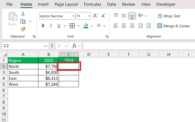
STEP 1: Open the Excel workbooks that you want to link.

STEP 2: In the cell where you want to insert the cross-reference, start by typing the equal sign = to begin your formula.

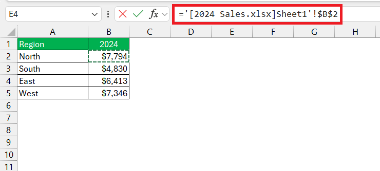
STEP 3: Navigate to the sheet that contains the data you want to cross-reference and click on the cell that has the data. You’ll notice that Excel automatically inputs the cell reference in your formula, which is prefaced by the sheet name.

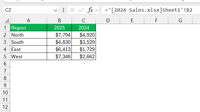
STEP 4: Press Enter.

The cell where you wrote the formula will now display the data from the cross-referenced cell. If the original data changes, the cross-referenced cell will update automatically. Remember, this basic link is relative by default; if you copy and paste the formula to another cell, Excel adjusts the reference.

 

Tools and Functions for Cross Referencing

Using VLOOKUP for Cross Referencing

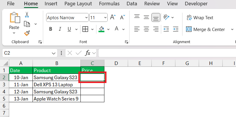
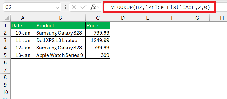
The VLOOKUP function is one of my go-to tools for cross-referencing. If I want to find the price of a product listed in another sheet, follow the steps below –

STEP 1: Go to the cell where I want the result.

STEP 2: Type the formula: =VLOOKUP(B2,’Price List’!A:B,2,0)

This formula searches for the value in B2 within Price List’!A:B and retrieves the corresponding value from the second column.

Using INDEX-MATCH for Cross-Referencing

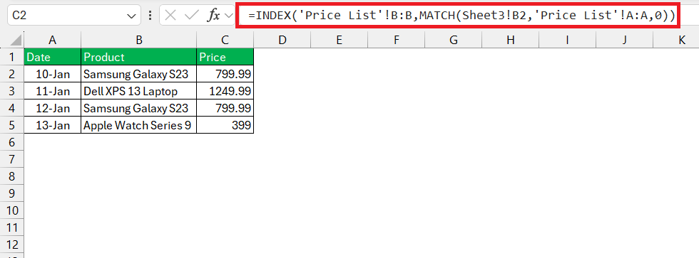
When I need more flexibility, I turn to the INDEX-MATCH combination. Unlike VLOOKUP, this method isn’t restricted to searching in the leftmost column.

If I need to find a sales rep’s name based on their ID, I will use the formula: =INDEX(‘Price List’!A:A,MATCH(Sheet3!B2,’Price List’!B:B,0))

Here, MATCH finds the row number of the ID in column A, and INDEX retrieves the corresponding value from column B.

 

Advanced Techniques: VLOOKUP and Beyond

Using Conditional Formatting for Cross-Referencing

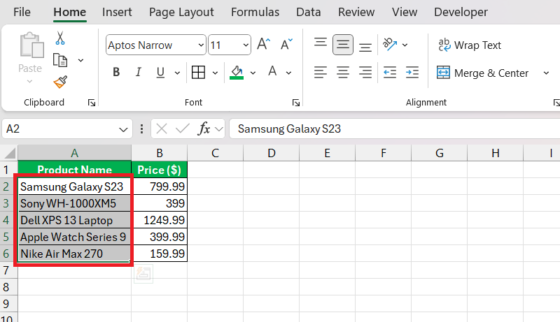
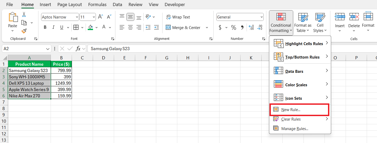
Conditional formatting is a visual way for me to highlight matches or discrepancies between datasets. I want to highlight items in one list that appear in another sheet, follow the steps below –

STEP 1: Select the range I want to format.

STEP 2: Go to Home > Conditional Formatting > New Rule.

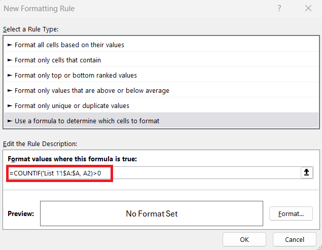
STEP 3: Select ‘Use a Formula to Determine Which Cells to Format’ and type this formula: =COUNTIF(Sheet2!A:A, A1)>0.

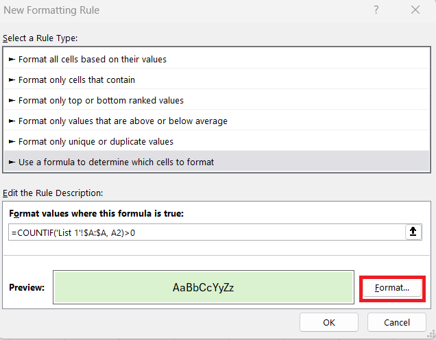
STEP 4: Choose a format, like a color fill, to highlight matches.

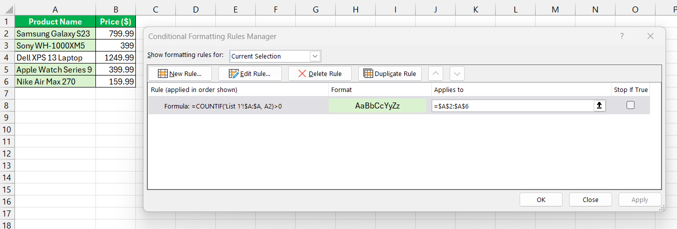
The matches will be highlighted.

Cross Referencing with Data Validation

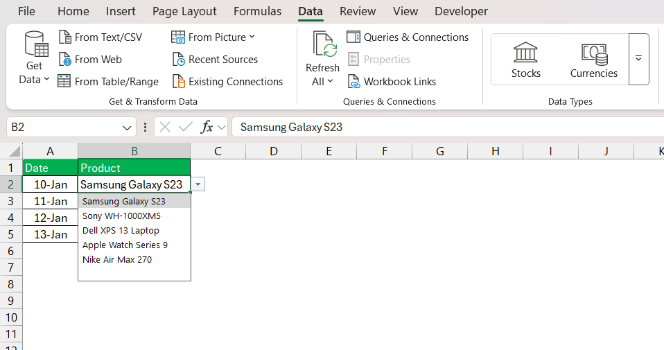
Data validation ensures that entries in one table match a predefined list. I’m creating a dropdown menu for product names based on another sheet.

STEP 1: Go to Data > Data Validation.

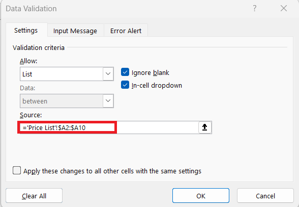
STEP 2: Select List and enter the source range (e.g., Price List!A:A).

This creates a dropdown menu with only valid options from the referenced list.

Tips for Effective Cross-Referencing

• Use Named Ranges: I often name ranges to make formulas easier to read and manage.
• Check for Errors: Functions like IFERROR or ISNA help me handle errors gracefully.
• Keep Data Organized: Consistent formatting and structured tables reduce errors during cross-referencing.

 

FAQ: Excel Cross Referencing

What is cross-reference in Excel?

In Excel, a cross-reference is a way to link and display information from one part of a workbook to another. By referencing cells across different sheets, I can create dynamic connections that automatically update when the source data changes. It’s a powerful tool for consolidating and analyzing data without duplicating it.

How Can I Ensure My Cross-References Stay Accurate During Collaborative Projects?

To keep cross-references accurate during collaborative projects, I use Excel’s ‘Track Changes’ feature and protect important cells. Sharing guidelines on data entry and formula usage with collaborators also helps maintain consistency. Regular audits for veracity are key.

What Are Some Common Mistakes to Avoid When Using Cross-Referencing In Excel?

Common mistakes to avoid in Excel cross-referencing include not using absolute references when necessary, mismatching data types, and overlooking errors from moved or deleted rows/columns. Always double-check references for accuracy.

Can I use these cross referencing techniques in mobile versions of Excel?

Yes, most cross-referencing techniques can be used on mobile versions of Excel. However, the interface is different and some advanced features may be limited, so ensure that the necessary functions are supported on your device.

What is a cell reference in Excel?

A cell reference in Excel is the unique identifier of a cell’s location in a worksheet, consisting of the column letter and row number, such as A1 or B2. It’s used to point to specific cells in formulas and functions for calculations and data analysis.