When you have an array of data in Excel you can quickly select an item and press the AutoFilter button which will filter that selection in your data.
You can then go over to another column within your data and select another item, apply the same steps above and further filter your data.
This is a quick and easy way to drill down into your data.
Download workbookFilter-by-Selection.xlsx
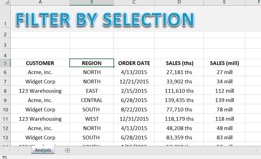
This is our data table.
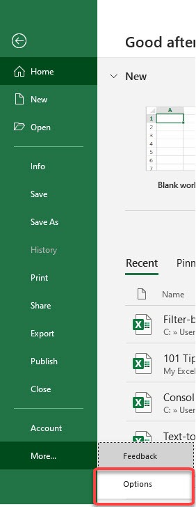
STEP 1: For this trick to work you need to put the AutoFilter button in the Quick Access Toolbar by going to File > More > Options > Quick Access Toolbar
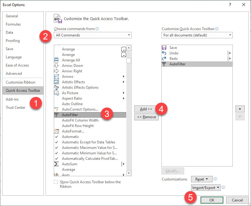
STEP 2: Then you need to go to Choose commands from > All Commands > AutoFilter > Add > OK
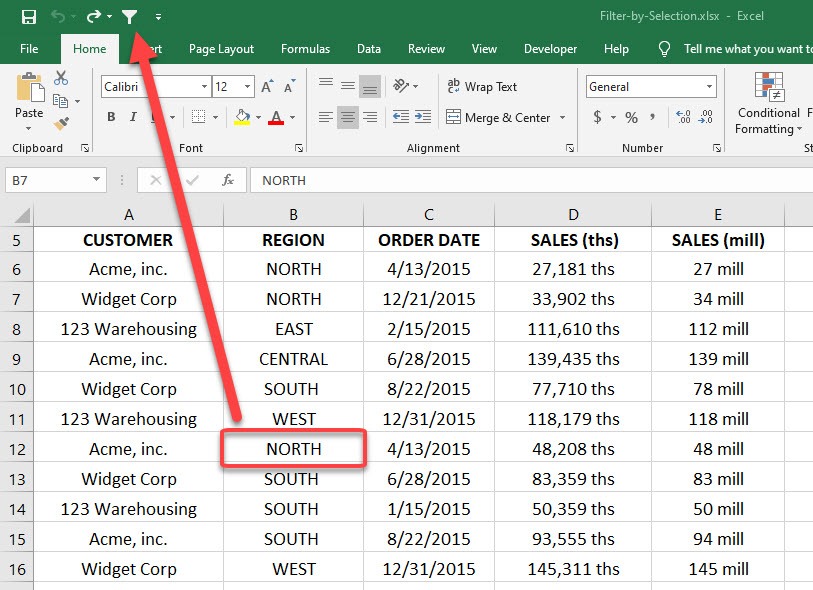
You can now see the AutoFilter icon on top.
STEP 3: You can then click anywhere in your data, click the AutoFilter button in your Quick Access Toolbar and see the magic!
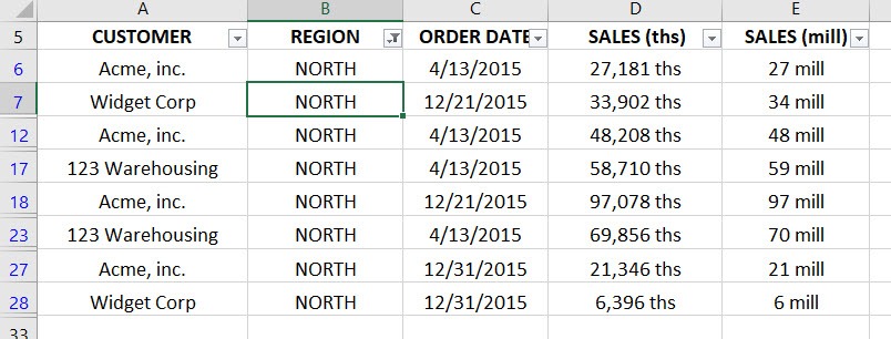
Let us say we want to filter the data by Region – North. Click on any NORTH value.
Afterwards click on the AutoFilter icon.
Your table is now filtered by the NORTH REGION with a single click!
John Michaloudis is a former accountant and finance analyst at General Electric, a Microsoft MVP since 2020, an Amazon #1 bestselling author of 4 Microsoft Excel books and teacher of Microsoft Excel & Office over at his flagship MyExcelOnline Academy Online Course.


