Top 7 Excel Interview Questions to Land Your Dream Job!

It is a must know software for anyone working on number crunching, data analysis, business reporting, charting, and various ad-hoc reports. If you are searching for a job that has “Microsoft Excel” as a prerequisite, you should be prepared to face a few Excel questions when you have your job interview.

Don’t be afraid as we are here to help you CRUSH these Excel interview questions!

This tutorial will guide you on the most popular Excel interview questions that will be asked by the interviewer when you are looking for jobs related to finance, accounting, auditing, budgeting, management, project management, administration, and sales, just to name a few.

Following are the Top 7 Excel interview questions that you need to prepare for to take you to the next round:

• #1 – VLOOKUP Function
• #2 – Freeze Panes
• #3 – Remove Duplicates
• #4 – Excel Tables
• #5 – Excel Pivot Tables
• #6 – Protect Sheets
• #7 – Merge Cells

For some bonus tips on crushing your Excel interview questions, listen to our podcast below to get the best Excel interview tips from the Excel experts and MVP’s around the world:

Let’s look at each of these topics one-by-one!

Before you proceed forward, make sure you download this Excel Workbook and follow along:

 

#1 – VLOOKUP Function

• What are the arguments of a VLOOKUP function?
• What are the limitations of this function?
• What are the alternate functions that can be used to overcome the limitations?

 

VLOOKUP is the most used function and hence is most likely to be asked in your Excel interview questions.

It is used to look up the value in the left-most column of the data table and returns a value in the same row from another column (to the right) in the table array.

 

The syntax of VLOOKUP is:

=VLOOKUP(lookup_value, table_array, col_index_num, [range_lookup])

where:

• lookup_value – the value you want to look for in the 1^st column of the data table
• table_array – the data table
• col_index_num – the column form which you want to derive the value
• [range_lookup] – Approximate match (TRUE) or Exact match (FALSE). The default value is TRUE. This is an optimal argument.

 

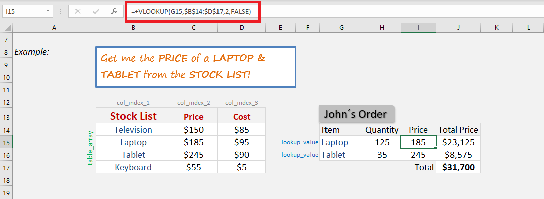
In the example below, we have used the VLOOKUP function to extract the price of the item from the stock list:

To learn about the different ways you can apply the VLOOKUP Function in Excel, CLICK HERE for Excel help!

 

The limitations of this function are:

• If the lookup value is not the 1st column of the data table, it cannot be used.
• If you add or delete columns in the data table, the function will produce the wrong results.
• Vlookup only finds the first match, ignores the rest.
• The default value of the range_lookup argument is an approximate match.
• Vlookup is not case-sensitive.

You can use either INDEX-MATCH or XLOOKUP to overcome these limitations. Learn more about these advanced functions and be prepared for your Excel interview questions.

 

#2 – Freeze Panes

• How to freeze top row or 1st column in Excel?
• How to fix column headings to keep them visible whilst we are scrolling down data?
• How to freeze multiple rows in Excel?

 

You can easily freeze top rows or columns in Excel by following the steps below:

Freeze Top Row

Go to View > Freeze Panes > Freeze Top Row

This will freeze the Row 1 of your sheet:

Try scrolling down, the first row is always visible!

 

Freeze First Column

To freeze the 1st column of your data, Go to View > Freeze Panes > Freeze First Column.

The first column of your data will be frozen!

 

Freeze Multiple Rows

If you wish to freeze multiple rows (say from Row 1 to 5), select the 6th row and then go to View > Freeze Panes > Freeze Panes.

This will freeze all rows above Row 6!

You can go through the tutorial on Excel freeze panes by Microsoft by Clicking Here.

 

#3 – Remove Duplicates

• How to get a unique list of customers from sales data?
• How to remove duplicate value from a column?

 

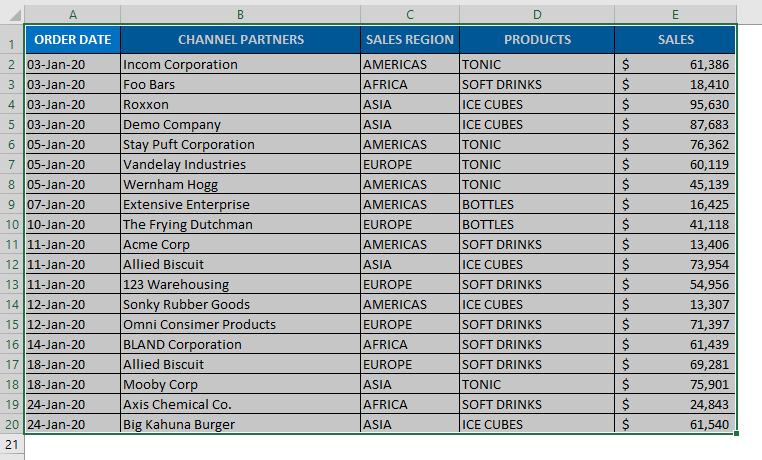
Let’s use an example to understand how to answer these Excel interview questions.

To remove duplicates from a set of data, follow the steps below:

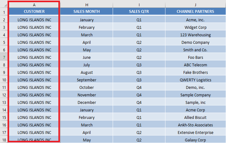
STEP 1: Select the column containing duplicate values.

 

STEP 2: Go to Data > Remove Duplicates.

 

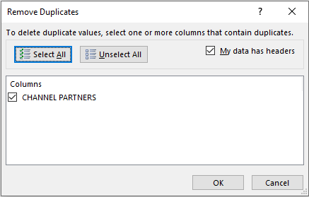
STEP 3: In the Remove Duplicates dialog box, make sure the box for  “My data has headers” is checked and click OK.

 

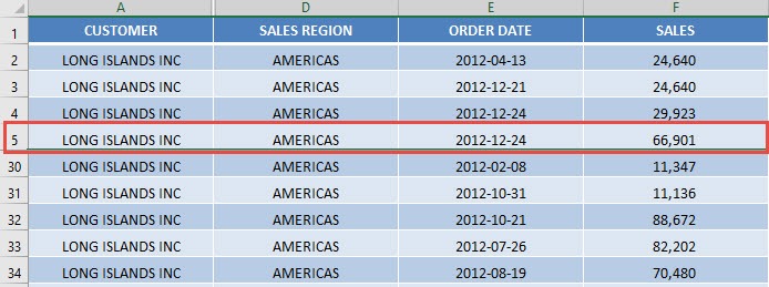
Excel will remove the duplicate values and provide you with a unique list!

 

#4 – Excel Tables

• How to convert a range of data into Excel Tables?
• What are the benefits of using an Excel Data Table?

 

Excel Tables are an excellent way to organize and analyze data accurately. It can be used to easily sort and filter data. There are numerous benefits of converting your data into Excel Tables

Converting a range into a formatted table can be done in a matter of seconds. Take the steps below to do so:

STEP 1: Select the Data.

STEP 2: Go to Insert > Table.

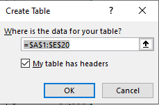
STEP 3: In the Create Table dialog box, Click OK. (Make sure you check the box next to My Data has headers)

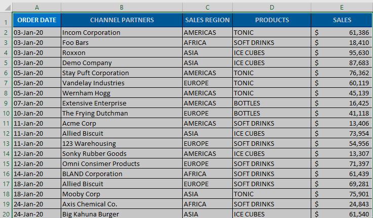
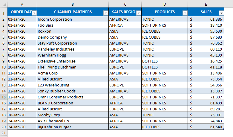
This is how your formatted Excel Data Tables looks like!

 

There are a plethora of benefits that you can utilize when you convert your data range into an Excel Table:

• Structured referencing;
• Many different built-in Table Styles with color formatting;
• Use of a “Total Row” which uses built-in functions to calculate the contents of a particular column;
• Dropdown lists that allow you to Sort & Filter;
• Insert interactive buttons or Slicers, to filter your Table’s data;
• When you scroll down from the Table, its Headers replace the Column Letters in the worksheet;
• Remove Duplicate Rows automatically;
• Summarize the Table with a Pivot Table;
• Supports calculated Columns so you can create dynamic formulas outside the Table;

 

#5 – Excel Pivot Tables

• What is an Excel Pivot Table?
• Why do you need an Excel Pivot Table?
• What are the features of Excel Pivot Tables?
• How can you filter data in Pivot Table?

 

If you want to analyze your data quickly (without using Formulas) and create informative reports, an Excel Pivot Table is your answer!

Pivot Tables in Excel are one of the most powerful features within Microsoft Excel.  It allows you to analyze more than 1 million rows of data with just a few mouse clicks and show the results in an easy to read table.

 

Follow the steps below to learn how to create Excel Pivot Table and answer those Excel interview questions like a pro:

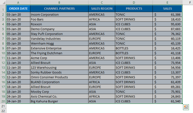
STEP 1: Select the Data.

STEP 2: Go to Insert > Pivot Table.

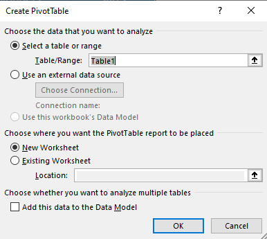
STEP 3: In the Create PivotTable dialog box, Click OK.
(Select whether you want Pivot Table in a New or Existing Worksheet)

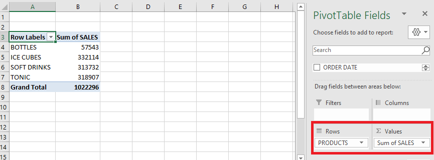
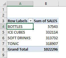
This will create a Pivot Table structure for you. Simply drag and drop fields in the row and values section and your Pivot is ready!

Click here to read about an interactive tutorial on the 50 different things you can do with an Excel Pivot Table!

 

Here are some of the advantages of using Pivot Table in your data:

• It is very easy to create a summary report of your data.
• It helps to analyze a large set of data with just a few clicks.
• You can create a report without writing any formulas.
• To see the transactions behind a Pivot Table value, simply double click on any value.
• You can insert inetractive buttons or Slicers to filter your data.
• You can add new data to your data source and Refresh your Pivot Table to see the new information in your Pivot Table report.

 

To filter data in the Pivot Table, simply create a Slicer:

STEP 1: Select a cell inside the Pivot Table.

STEP 2: Go to PivotTable Analyze > Insert Slicer.

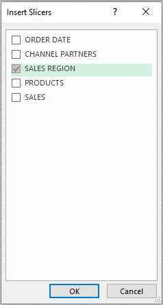
STEP 3: In the Insert Slicers dialog box, select the checkboxes next to the column (Sales Region)  you want to display as a filter.

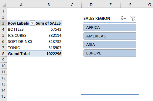
An Excel Slicer will be created for the fields (Sales Region) you have selected above.

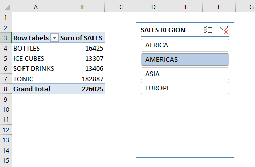
STEP 4: Select Americas to filter the data for that particular item.
The data has been filtered!

 

#6 – Protect Sheets

• How to protect sheets in Excel?
• How to secure formulas in your Excel sheet?

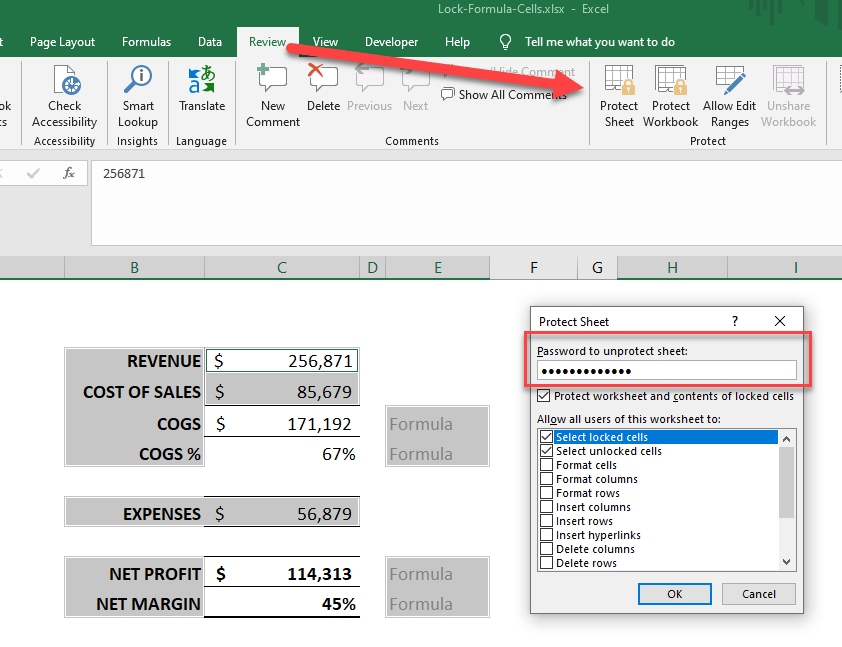
If you have lots of formulas in your Excel Worksheet and you want to secure those formulas, you can protect your sheets. To protect sheets in Excel, follow the steps below:

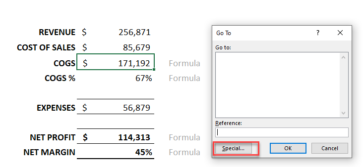
STEP 1: Press the Go To Special shortcut CTRL+G

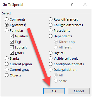
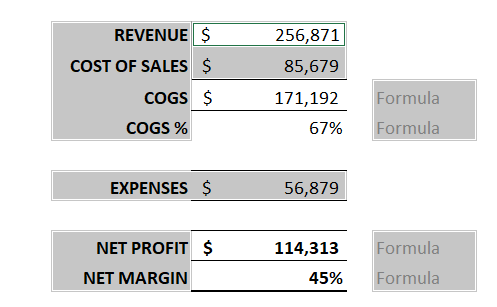
STEP 2: Select the Constants box and press OK (this highlights all the non-formula cells)

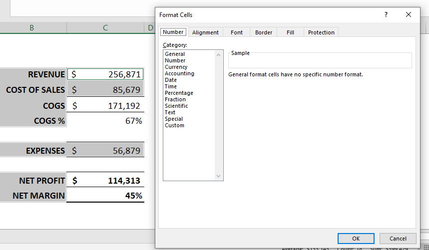
STEP 3: Press CTRL+1 to bring up the Format Cells dialogue box

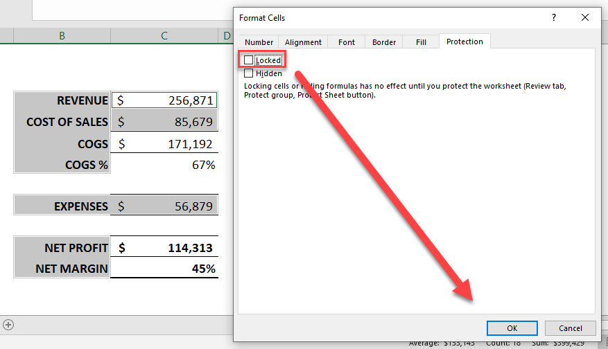
STEP 4: Select the Protection tab and Un-check the Locked box

STEP 5: Go to Review > Protect Sheet > then enter your custom password (optional)

This will lock all the cells that are not constant, so all the formula cells 🙂

To know more about how to protect your sheet and to ace that Excel practice test, Click Here!

 

#7 – Merge Cells

• How to merge cells in Excel?
• How to combine multiple cells in Excel?

A great way to customize the layout of your Excel worksheet is to merge multiple cells into one cell.

 

Follow the steps below to learn how to answer this Excel interview question on Excel merged cells:

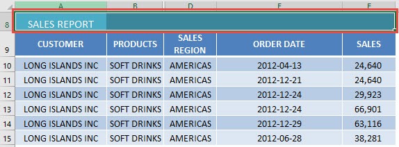
STEP 1: Make sure to select all of the cells you want to merge together:

 

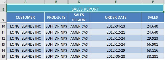
STEP 2: Go to Home > Alignment > Merge & Center

The top row is now merged together!

Excel has a number of approaches on how to merge cells in Excel that spans across rows and/or columns. Click here to learn more about it and answer those Excel questions by the interviewer with confidence.

 

Conclusion

In this article, you have been provided with a detailed guide on the frequently asked Microsoft Excel interview questions and answers in any Excel practice test.

There are many important features in Excel that you must be prepared for before sitting for an interview. You can learn more about how to use Excel by viewing our FREE Excel webinar training on Formulas, Pivot Tables, and Macros & VBA!

Go through these Excel help tutorials to gauge your Excel skills and crush your Excel interview questions so that you can land your dream job.

For some bonus tips on crushing your Excel interview questions, listen to our podcast below to get the best Excel interview tips from the Excel experts and MVP’s around the world: