Named Ranges with Vlookup Formula

A Named Range makes it easier to understand Excel formulas, especially if the said formula contains an array argument. A Named Range can be a cell, a cell range, a Table, a function, or a constant.

Key Takeaways:

• Improves Formula Readability: Using named ranges in a VLOOKUP formula makes it more readable and easier to understand. For example, =VLOOKUP(A2, SalesData, 2, FALSE) is more intuitive than using a range reference like =VLOOKUP(A2, A1:D10, 2, FALSE).
• Simplifies Range Updates: Named ranges allow you to update the data range in one place without needing to adjust multiple formulas. If the range for “SalesData” changes, updating the named range automatically reflects in all related formulas.
• Enhances Formula Management: Named ranges help reduce errors by eliminating the need to manually adjust cell references in complex or frequently used VLOOKUP formulas.
• Dynamic Named Ranges for Flexibility: Combining named ranges with dynamic formulas like OFFSET or INDEX makes VLOOKUP more powerful. These dynamic ranges automatically adjust as data expands or shrinks.
• Named Ranges Across Sheets: Named ranges can be defined across different worksheets, allowing VLOOKUP to easily reference data from other sheets without manually specifying the sheet name in the formula.

 

What does it do?

Searches for a value in the first column of a table array and returns a value in the same row from another column (to the right) in the table array.

Formula breakdown:

=VLOOKUP(lookup_value, table_array, col_index_num, [range_lookup])

What it means:

=VLOOKUP(this value, in this Named Range, and get me value in this column, Exact Match/FALSE/0])

 

How to Use Named Ranges with Vlookup Formula

STEP 1: To define a Named Range in Excel you need to select the cell/cell range/Table/function/constant and go to the Name Box which is located on the top left-hand corner of the workbook – next to the Formula Bar.

 

STEP 2: In here you can name your range whatever you like (make sure there are no spaces) and press Enter.  You can view your Named Range by clicking on the drop-down box in the Name Box.  In our example, we will give this a name of StockList.

You can also view/edit/delete your Named Range by going to the Formulas tab in the Ribbon menu and selecting Name Manager.

 

STEP 3: Now that you are all set, each time you are creating a formula, like a Vlookup formula, it is best to use a Named Range as it makes the formula easier to understand and maintain.

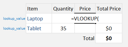
We need to enter the Vlookup function:

=VLOOKUP(

The Vlookup arguments:

lookup_value

What are we looking for?

Reference the cell that contains the text or value:

=VLOOKUP(G15,

table_array

From which list are we doing a lookup on?

The formula for Excel VlookUp Named Range will be:

=VLOOKUP(G15, StockList,

col_index_num

From which column do we want to retrieve the value?

We want to retrieve the Price which is the SECOND column from our table array:

=VLOOKUP(G15, StockList, 2,

[range_lookup]

Do we want an exact match?

Place in FALSE to signify that we want an exact match:

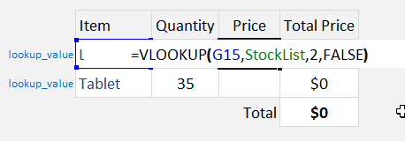
=VLOOKUP(G15, StockList, 2, FALSE)

This is how the price will now dynamically change based on your selection with Vlookup using named range:

Frequently Asked Questions:

What are the benefits of using named ranges with the VLOOKUP formula?
Named ranges improve formula readability and make it easier to manage data ranges. Instead of referencing a cell range like A1:D10, you can use a named range like SalesData, which simplifies your formula and reduces errors when ranges need updating.

How do I create a named range for use in a VLOOKUP formula?
To create a named range, select the range of cells you want to name, go to Formulas > Define Name, enter a name (e.g., “SalesData”), and click OK. You can then use this name in your VLOOKUP formula, such as =VLOOKUP(A2, SalesData, 2, FALSE).

Can I use dynamic named ranges with the VLOOKUP formula?
Yes, you can use dynamic named ranges created with formulas like OFFSET or INDEX. For example, define a named range using a formula like =OFFSET(Sheet1!$A$1, 0, 0, COUNTA(Sheet1!$A:$A), 4), which automatically adjusts as new data is added. Then, use this named range in VLOOKUP.

Can a named range reference data on a different sheet for VLOOKUP?
Yes, named ranges can reference data on other sheets. Simply define the named range to include the data from the other sheet (e.g., Sheet2!A1:D10), and use it in your VLOOKUP formula. The formula will work without needing to specify the sheet name directly.

What should I do if VLOOKUP with a named range is returning #N/A?
If VLOOKUP returns #N/A, check that the lookup value exists in the first column of the named range. Also, ensure the named range includes the necessary data, and verify that you’re using the correct column index and an appropriate match type (e.g., FALSE for an exact match).