How to Optimize Data with the Excel Rank Function

If you’ve ever worked with a large dataset in Excel and needed to rank values, you know it can be time-consuming. That’s where Excel RANK function comes in handy! In this article, I’ll guide you through what the RANK function does, how it works, and some practical examples to get you started.

Key Takeaways:

• The RANK function efficiently determines the rank of a value within a dataset, either in ascending or descending order.
• Understanding syntax like RANK(number, array, [order]) helps tailor rankings to specific needs.
• Advanced techniques, like using RANK.EQ, RANK.AVG, or combining COUNTIF, handle ties effectively.
• Common pitfalls include incorrect range references and mishandling ties, which can distort analysis.
• The RANK function saves time, enhances data insights, and simplifies large dataset comparisons.

 

Introduction to Excel Rank Function

What is the RANK Function?

The RANK function in Excel is used to determine the rank of a specific value within a list of values. It assigns a rank to each number in a dataset, making it easy to see how each value compares to the others. The function can rank values in either ascending or descending order, depending on my needs.

Why Mastering the Rank Function Is Essential

Mastering the Rank function in Excel is essential because it allows us to quickly assess and compare the relative standing of numbers in a dataset. We can use it in various contexts, from educational settings where we evaluate student performance, to business environments where sales figures or performance metrics need to be sorted and sifted through.

By efficiently ranking data, we can discern top performers, identify outliers, and prioritize efforts. Learning how to apply this function can save us hours of manual comparison and sort activities and facilitate a deeper understanding of large datasets that inform strategic decisions.

 

Grasping the Rank Function Basics

Syntax and Parameters for Using the Rank Function Effectively

To use the Rank function effectively in Excel, it’s important to understand its syntax and parameters. The syntax for the Rank function is:

RANK(number, array, [order])

Where:

• number is the value to find the rank for.
• array is the range of data within which we want to rank number.
• [order] is an optional argument; if 0 (or omitted), it ranks number in descending order (highest to lowest), and if 1, it ranks in ascending order (lowest to highest).

To utilize this function to full effect, ensure that number is a part of the array specified, as the function looks for the number within that array to determine its rank. Also, the [order] parameter is crucial when the direction of ranking matters for your analysis.

Omitting it or using 0 will place the higher values at the top, while using 1 does the opposite, which is particularly useful when dealing with times in a race, cost units, or instances where lower numbers are preferable.

By using the appropriate combination of these parameters, we can gather meaningful insights and patterns from our dataset, which would otherwise remain obscured.

 

Step-by-Step Examples

Example 1: Ranking Sales Figures in a Dataset

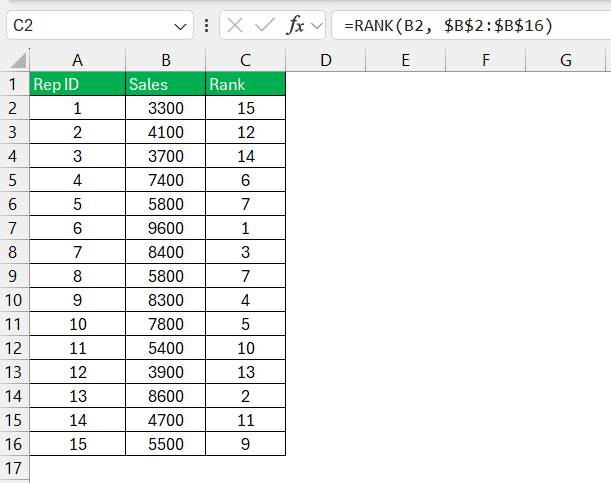
Let’s take a practical dive into using Excel’s RANK() function to rank sales figures in a dataset. We have a list of salespeople with their respective monthly sales. To rank these figures from highest to lowest, we’ll apply the formula: =RANK(B2, $B$2:$B$16) in the adjacent cell and drag it down to apply it to each salesperson’s figures.

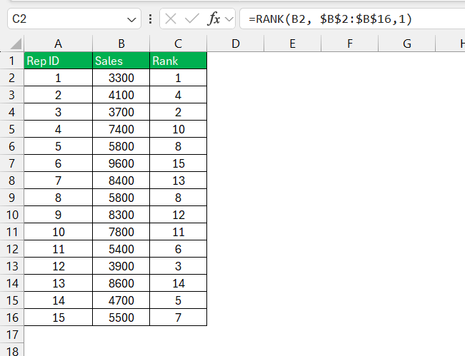
Upon completion, we’ll have implemented the rankings for the whole team. If we wish to rank in ascending order (for different metrics where lower is better), we’d use: =RANK(B2, $B$2:$B$16, 1).

After ranking, we can better assess who’s leading sales and who needs further support to meet their targets, facilitating targeted management and training approaches.

Example 2: Analyzing and Adjusting Race Times

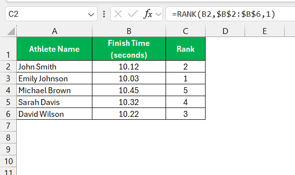
Racing times provide a vivid example of how efficiently the Rank function can be leveraged. Imagine we have a list of athletes with their respective finish times from a 100-meter dash, and we need to rank these times in ascending order—where the smallest time is the fastest.

Using the Rank function, we apply: =RANK(B2,$B$2:$B$6,1) beside each athlete’s time. This ranks their performance with the number 1 assigned to the fastest time and ascending from there.

Utilizing the function in this way ensures that the ranks reflect the true outcomes of the race, facilitating accurate analysis and a clear display of athletic performances.

 

Advanced Techniques with Rank Function

Using RANK.EQ and RANK.AVG

Excel also offers two additional ranking functions: RANK.EQ and RANK.AVG. These functions provide more options for handling ties.

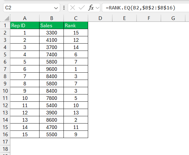
RANK.EQ: This function works similarly to the RANK function, assigning the same rank to tied values. The syntax is the same as the RANK function:

=RANK.EQ(number, ref, [order])

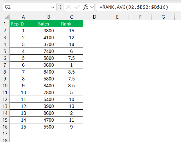
RANK.AVG: This function assigns the average rank to tied values. For example, if two values are tied for third place, they both receive a rank of 3.5. The syntax is:

=RANK.AVG(number, ref, [order])

Handling Ties

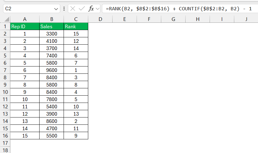
One thing I’ve noticed when using the RANK function is that it assigns the same rank to tied values. For example, if two sales figures are the same, they both get the same rank, and the next rank is skipped. While this is usually acceptable, there are times when I need unique ranks. To achieve this, I can use a combination of the RANK function and the COUNTIF function.

For example, if I have sales figures in column A and ranks in column B, I use the following formula in cell B2:

=RANK(A2, $A$2:$A$10) + COUNTIF($A$2:A2, A2) – 1

I use the COUNTIF function to count how many times each rank appears before the current value. By adding this count minus one to the rank, I ensure unique ranks for tied values.

 

Common Pitfalls and How to Avoid Them

The Risks of Incorrect Range References and Ignoring Ties

Dealing with incorrect range references is a common pitfall in Excel that can lead to skewed data and subsequent analysis. If, for example, we add new data to a dataset but fail to update the range in our Rank formula, this could result in an incomplete overview, as the new data points aren’t considered in the rankings. It’s imperative to regularly check and update ranges in our formulas to include all relevant data.

Ignoring ties is another risk that can distort the outcomes of our analysis. If a dataset contains duplicate values, use RANK or RANK.EQ without due consideration for how ties are treated can lead to misleading ranks. Deciding how to handle ties—whether by assigning them the same rank or averaging their ranks—can significantly affect subsequent data interpretation and the decisions made based on it.

Regular vigilance in managing these aspects ensures data integrity and maintains the reliability of our analysis.

FAQs

How do you use the rank function in Excel?

To use the rank function in Excel, input =RANK(number, reference, [order]) into a cell. Replace number with the cell containing the value you want to rank, reference with the range of cells to rank against, and [order] with 0 for descending or 1 for ascending order. Remember, the [order] argument is optional, and the default is descending.

How Do You Use the Rank Function for Non-Adjacent Cells?

To rank non-adjacent cells in Excel, you must enter the cell references separated by commas into the rank function and enclose them in parentheses. For instance, =RANK(B2, (B2, D2, F2)). Make sure to lock the references with the $ sign if you plan to copy the formula across columns or rows.

Can You Rank Text Values Alongside Numbers?

No, you cannot directly rank text values using the RANK() function because it’s designed for numeric values only. If you need to rank a mix of text and numbers, consider assigning numeric equivalents to text categories, then using the RANK() function on those numbers.

What’s the Difference Between the RANK and RANK.EQ Functions?

There is no difference between the RANK and RANK.EQ functions; they both operate identically by assigning the same rank to tied numerical values and skipping subsequent ranks. RANK.EQ was introduced for clarity, as RANK may eventually be phased out for consistency in Excel’s function naming conventions. It’s generally recommended to use RANK.EQ in the newer versions of Excel to future-proof your worksheets.

How Does the COUNTIF Function Aid in Ranking Tied Data?

COUNTIF helps in ranking tied data by determining the count of entries that tie with a certain value and those that surpass it. When used in combination with RANK or RANK.EQ, it can break ties based on a secondary criterion. It modifies the rank number slightly to account for the presence of higher or additional qualifying scores in the data set, ensuring each tie is fairly addressed.