Unlock the full potential of your Excel spreadsheets with our concise guide on Row & Column Freeze. Turn navigating through vast data sets into a breeze by keeping crucial information in sight at all times. Whether you’re a novice or an Excel veteran, our step-by-step instructions and practical examples will transform the way you manage and analyze data.
Key Takeaways
- Freezing headers or vital data points in Excel maintains visibility, improving data comprehension and analysis efficiency.
- Consider spreadsheet size and freeze multiple rows if needed to keep important details accessible during data navigation.
- By pressing Alt+W, F, F, you quickly summon the Freeze Panes command without removing your hands from the keyboard.
Table of Contents
Introduction: Simplifying Excel Operations
The Need for Efficiency in Excel Navigation
If you’ve ever found yourself lost scrolling through an extensive Excel spreadsheet, you’re not alone. Efficiency in navigating Excel is crucial, whether you’re analyzing data, balancing budgets, or tracking inventory. Understanding how to quickly access the data you need without losing sight of your headers can turn a frustrating task into a smooth, productive experience.
Freezing Rows and Columns Quickly
Mastering the Freeze Panes Feature in a Minute
Learning to use the Freeze Panes feature in Excel can greatly enhance your ability to analyze data without the annoyance of endless scrolling. In just a minute, you can master this simple yet powerful tool and keep your important rows or columns visible while you work on the rest of your spreadsheet.
By utilizing this feature, you enable a static view of specified areas of your sheet, which is especially useful in large workbooks. Once you get the hang of it, freeze panes will be an indispensable part of your Excel toolkit.
Shortcut Keys to Speed Up Your Workflow
Using keyboard shortcuts in Excel isn’t just a neat trick; it’s a productivity superpower. By pressing Alt+W, F, F, you quickly summon the Freeze Panes command without removing your hands from the keyboard.
Step-by-Step Guide to Row & Column Freeze
How to Freeze the Top Row with One Click
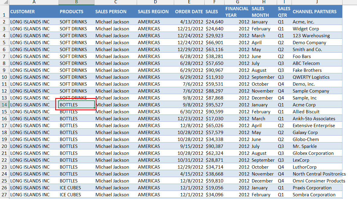
Freezing the top row in Excel is as straightforward as it gets, and with a single click, you can keep your headers in place while you navigate through your data.
STEP 1: Launch the Excel application and access your workbook.
STEP 2: Click the “View” tab to reveal the ribbon.
STEP 3: Locate and click on “Freeze Panes.”
STEP 4: From the dropdown, select “Freeze Top Row.”
That’s it! The top row is now frozen, and as you scroll down, you’ll always have a view of your column headings.
Locking the First Column in Less Than a Minute
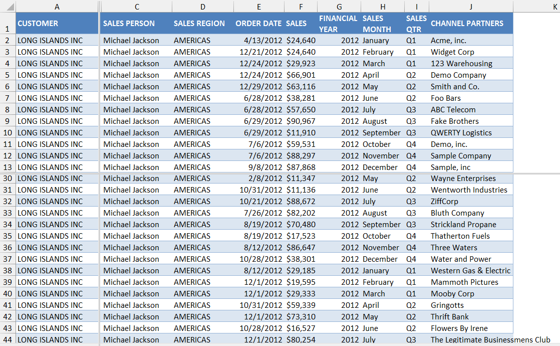
Locking the first column in your Excel spreadsheet can be accomplished quickly, ensuring that your leftmost data stays in view as you scroll horizontally.
To do this:
STEP 1: Open the Excel worksheet.
STEP 2: Go to the Excel Ribbon and select the “View” section.
STEP 3: Click on “Freeze Panes” to reveal the options.
STEP 4: Select “Freeze First Column” from the list.
The faint line appearing after column A indicates that the first column is now frozen. No matter where you navigate to the right, you can always see the first column clearly.
Unlocking the Potential of Frozen Panes
Utilizing Frozen Panes for Effective Data Comparison
Frozen panes can be an analysis game-changer in Excel, offering a simple way to compare diverse sets of data. By freezing rows or columns, you lock specific data points in place, enabling you to scroll through other parts of your spreadsheet without losing reference points.
For instance, if you’re comparing monthly financials, you might freeze the top row to keep the month names in view. As you scroll down through the figures, you’ll effortlessly remember which column correlates to which month. This is a particularly handy approach for longitudinal studies or when tracking variations over time.
Restoring to Default View Effortlessly
If you need to return to the default view in Excel without any frozen panes, restoring this setting is a breeze:
STEP 1: Click anywhere on your worksheet to ensure it’s active.
STEP 2: Head over to the “View” tab on the Excel Ribbon.
STEP 3: In the “Window” group, find and click on “Freeze Panes.”
STEP 4: Now simply select “Unfreeze Panes” from the dropdown menu.
Viola! Your Excel sheet will now return to its unfrozen state, allowing you to scroll freely through the entire worksheet with no locked rows or columns. Remember, freezing panes is not a permanent action—any adjustments can be reversed with just a few clicks.
Troubleshooting Common Issues
Addressing Problems with Freeze Panes Not Working
Occasionally, you may run into issues where the Freeze Panes feature is not working as expected. If the “Freeze Panes” button is grayed out, or your rows and columns aren’t freezing correctly.
Here are a couple of steps you can take:
- Exit Cell Editing Mode: If you’re entering data or a formula in a cell, Excel won’t allow you to freeze panes. Simply press ‘Enter’ or ‘Esc’ to exit the cell, and then try freezing your panes again.
- Check for Worksheet Protection: If your worksheet is protected, you won’t be able to use the Freeze Panes feature. Go to the “Review” tab, and click on “Unprotect Sheet” to remove protection.
Always ensure that you have the correct cell selected before you try to freeze panes, as this could also affect the outcome. By addressing these common issues, you can regain control and resume using the Freeze Panes function to enhance your productivity in Excel.
Splitting Panes for Alternative View Options
Splitting panes in Excel offers an alternative to freezing rows and columns, allowing you to divide your worksheet into separate scrollable areas for more dynamic comparisons or reviews of your data.
To split panes:
STEP 1: Open your Excel workbook and go to the worksheet you want to split.
STEP 2: Place your cursor in the cell where you want the split to occur. The panes will divide, appearing both above and to the left of the chosen cell.
STEP 3: Select the “View” tab located on the Excel Ribbon.
STEP 4: Select “Split” in the “Window” group.
This will create two or four separate scrollable areas, depending on where you’ve placed your cursor.
Splitting panes is a powerful tool that can make your data analysis more flexible, especially when you need to scroll independently through different parts of your sheet. To remove the split, simply click “Split” again, and the areas will merge back into a single pane.
Tips and Tricks
Freezing Multiple Rows or Columns Simultaneously
Freezing multiple rows or columns at the same time in Excel is a practical way to keep several header rows or columns static while you examine the rest of your data. Here’s a quick guide to freeze multiple panes simultaneously:
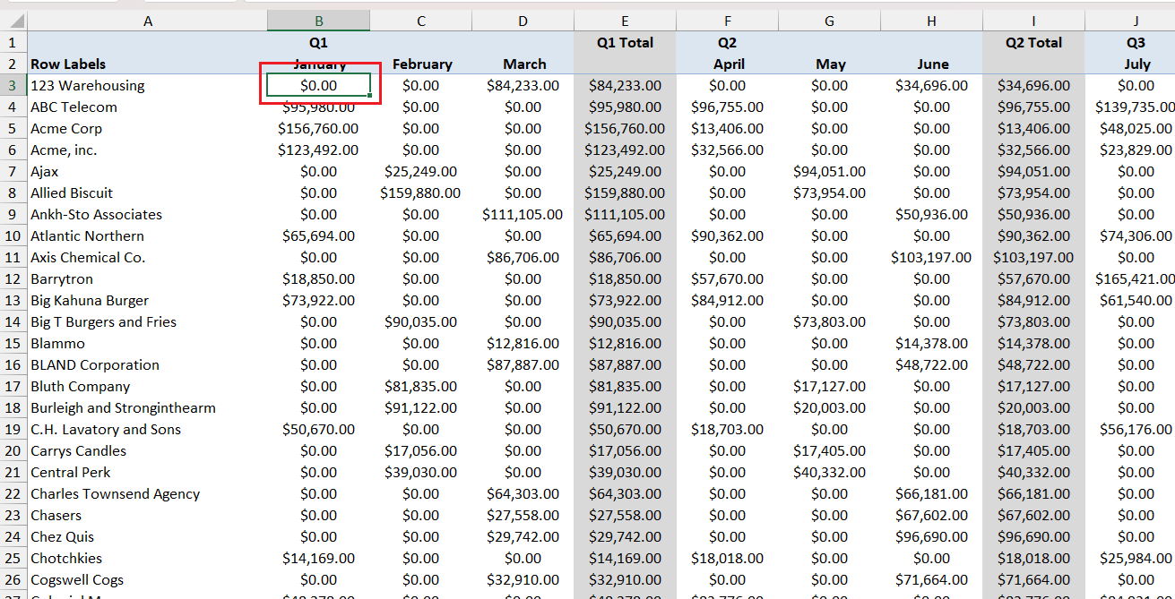
STEP 1: To freeze both rows and columns, select the cell below and to the right of where you want the split to happen. To lock the initial two rows along with a single column in place, select the cell located at B3.
STEP 2: Go to the “View” tab on the Excel Ribbon.
STEP 3: Click on “Freeze Panes” in the “Window” group.
STEP 4: Then choose “Freeze Panes” from the dropdown menu.
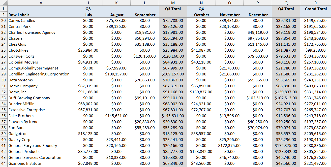
It’s worth noting that the panes will freeze above and to the left of the selected cell. The lines marking the frozen panes might appear thicker, indicating the division between frozen and scrollable areas of your worksheet.
FAQs
How to Quickly Freeze or Unfreeze Panes in Excel?
To quickly freeze panes in Excel, select the cell below and to the right of where you want the panes frozen. Then head to the “View” tab, click “Freeze Panes” in the “Window” group, and choose “Freeze Panes” from the dropdown. For unfreezing, return to the “View” tab, click “Freeze Panes,” and select “Unfreeze Panes.”
How do I freeze a specific row in Excel?
To freeze a specific row in Excel, click on the cell in the row directly below the one you want to freeze. Then navigate to the “View” tab, select “Freeze Panes” from the “Window” group, and click “Freeze Panes” in the dropdown menu. Your chosen row and all rows above it will be frozen.
How can I freeze a column?
To freeze a column in Excel, select the column to the right of the column you want to freeze. Go to the “View” tab, click on “Freeze Panes,” and then choose “Freeze Panes” from the dropdown. The column to the left will be frozen, along with any columns to its left.
Can You Freeze Multiple Rows and Columns at the Same Time?
Yes, you can freeze multiple rows and columns at the same time in Excel. Select the cell immediately below the rows and to the right of the columns you want frozen, navigate to the “View” tab, click “Freeze Panes,” and then choose “Freeze Panes” from the dropdown list.
John Michaloudis is a former accountant and finance analyst at General Electric, a Microsoft MVP since 2020, an Amazon #1 bestselling author of 4 Microsoft Excel books and teacher of Microsoft Excel & Office over at his flagship MyExcelOnline Academy Online Course.

