Expand and Collapse buttons in Excel Pivot Tables

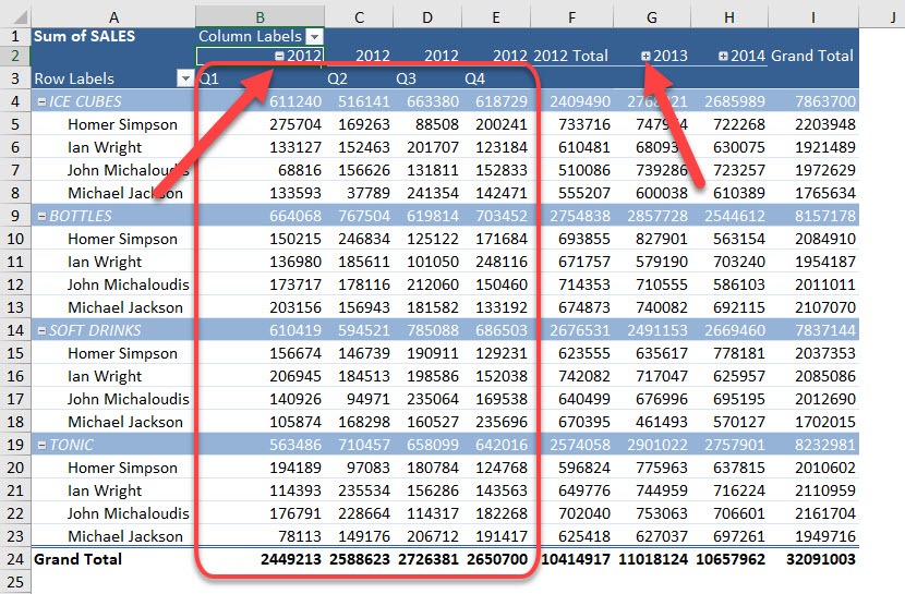
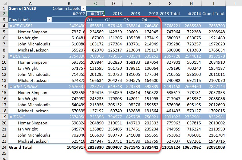
I will show you quickly how to use that for your Pivot Table rows and columns.

Exercise Workbook:

---

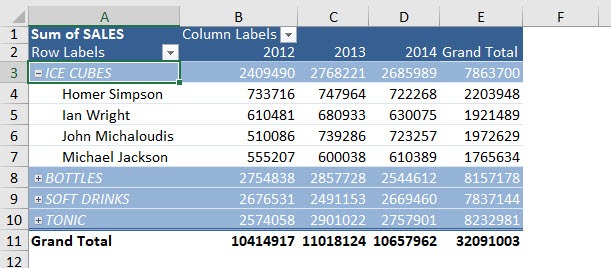
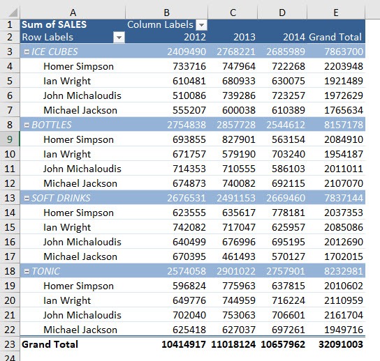
Here is our Pivot Table.

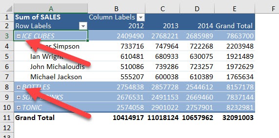
STEP 1: You can quickly click on the – button to collapse the Product Field, or the + button to expand the Product Field. Give it a try!

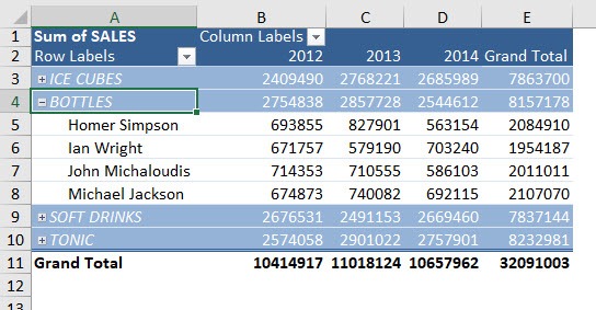
You can see the ICE CUBES is now collapsed, while BOTTLES has expanded.

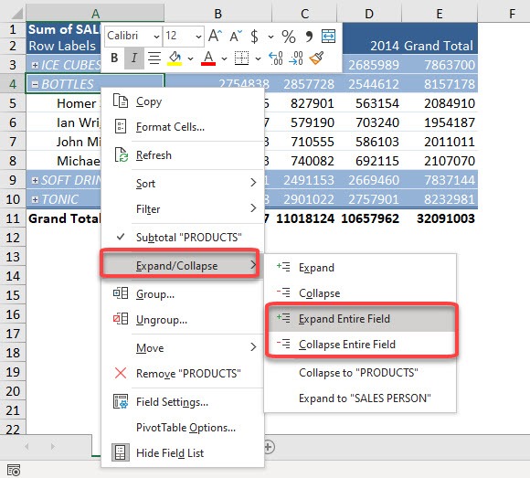
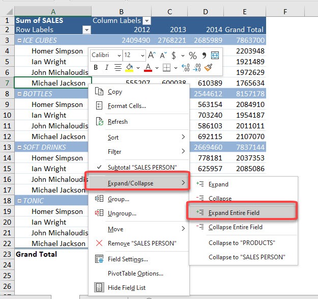
STEP 2: If you want this change to happen for all of the Products, right-click on a Product Field (Bottles) and select Expand/Collapse > Expand Entire Field

You can select the Collapse Entire Field option instead if you want to collapse all of the Product Fields.

All of the Products are now expanded!

STEP 3: What if we want to expand the Salesperson field? Right-click on any Salesperson and select Expand/Collapse > Expand Entire Field

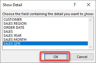
STEP 4: You will get a selection to add that detail under the Salesperson field. Select SALES QTR and click OK

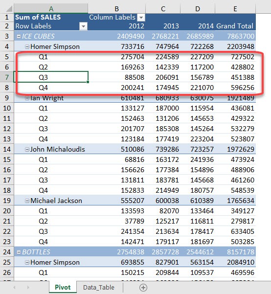
STEP 5: Now you have an additional level of detail (Sales Quarter) under Salesperson for your analysis!

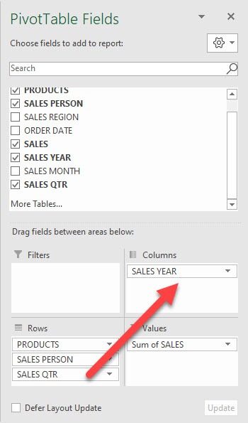
You have the same functionality for columns as well, drag the SALES QTR field from Rows to Columns

STEP 6: Now our column of Sales Year now has the additional detail of Sales Quarters.

You can quickly click on the – button to collapse the Sales Year Field, or the + button to expand the Sales Year Field.

You can now see we have collapsed the 2012 column while expanding the 2013 column using expand and collapse buttons.

 

Click here to learn all about Excel Pivot Tables!

 

Make sure to download our FREE PDF on the 333 Excel keyboard Shortcuts here: