How to Extract Cell Value with Excel Formulas and Functions

Unlocking the full potential of Microsoft Excel hinges on mastering the art of cell value extraction, a fundamental skill for data manipulation and analysis. By understanding the basics of Excel formulas and functions, users can harness its power to seamlessly navigate through vast datasets, making data-driven decisions with precision and efficiency.

Key Takeaways:

• Excel Formulas & Functions: They’re like simple equations, driving data manipulation on worksheets.
• Value Extraction Toolkit: Functions like VALUE, CELL, INDEX, MATCH, INDIRECT, and ADDRESS make extracting precise information effortless.
• Demystifying CELL: This function retrieves specific cell details, enriching users’ data comprehension.
• Power of INDEX & MATCH: Together, they offer flexibility and accuracy in retrieving data from large datasets.
• Dynamic Cell References: INDIRECT and ADDRESS adapt to changing data, boosting spreadsheet efficiency.

 

Mastering the Art of Cell Value Extraction in Excel

Understanding the Basics of Excel Formulas and Functions

When you’re learning to extract cell value in Excel, it’s crucial to start with the fundamentals. Excel formulas and functions are the building blocks that allow you to manipulate data with ease. Think of formulas as simple equations that perform calculations or operations on your worksheet data. They can be as straightforward as adding two numbers together, or as complex as pulling information from different data sets based on multiple criteria.

Understanding how to use these tools effectively can transform how you approach data analysis. Excel becomes a powerful ally, doing the heavy lifting for you, whether you’re averaging sales figures, summing expenses, or searching for specific data points.

The Essential Toolkit for Extracting Values

To deftly navigate the seas of data in Excel and extract the values you need, there’s an essential toolkit every user should be familiar with. These tools are the functions and features that enable you to pull data from cells and ranges with precision:

1. VALUE Function: Transforms text that looks like a number (including dates or times) into an actual numeric value.
2. CELL Function: Provides information about the formatting, location, or contents of a specific cell.
3. INDEX and MATCH: A powerful combination that retrieves the value at a particular position in a table or range, based on specific criteria.
4. INDIRECT: Converts a text string into a cell reference.
5. ADDRESS: Generates a cell address (as text) from specified row and column numbers.

These functions serve as your go-to toolkit for most of the data extraction tasks you’ll perform in Excel. They can be used in isolation or combined to create powerful formulas that delve into your data’s deepest layers to extract the gems hidden within.

 

Unlocking the Potential of Key Excel Functions

Demystifying the CELL Function

The CELL function may seem enigmatic at first glance, but once understood, it becomes a useful tool in your Excel skills inventory. The primary purpose of the CELL function is to retrieve specific information about a cell’s formatting, content, or environment.

As you’ve learned, this function uses two arguments: info_type and reference. The info_type lets you specify the kind of information you wish to extract about a cell, such as whether the content is a numeric value or text, the address, width, or even the file path if needed. The reference is the particular cell you’re interested in.

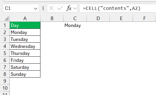
Here’s an example of its syntax: =CELL("contents", A2)

So, the formula returns the actual value or formula contained in cell A2. If cell A2 contains a formula, the function will return the formula itself. If cell A2 contains a value, it will return that value.

 

VALUE Function

• Usage: Use VALUE to convert text that appears in a recognizable numeric format into a number.
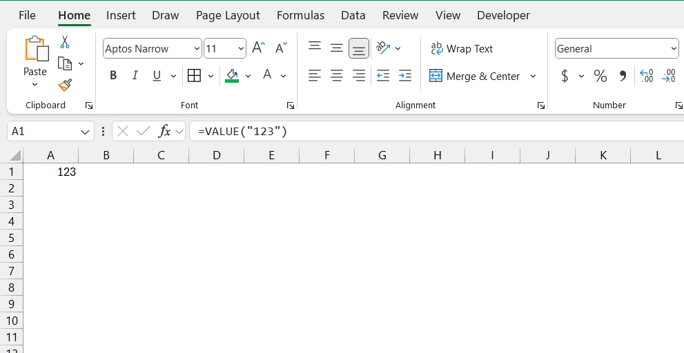
• Syntax: =VALUE(text)text can be a string within quotation marks or a cell reference containing the text to convert.

For example, =VALUE("123") will return 123 as a number.

These functions can be instrumental when working with imported data, where ensuring data types are correct is crucial before performing calculations. Remember, while VALUE is more about conversion, CELL is about information— each function yielding insights needed to refine and perfect your data management process.

 

The Power of INDEX and MATCH Functions

If you’re looking to harness Excel’s full potential, getting familiar with INDEX and MATCH functions is a game changer. These functions, when used together, form a robust alternative to the more widely known VLOOKUP or HLOOKUP functions, especially since they provide additional flexibility.

The INDEX function, simply put, returns a value from a specific place in a table or range. Its power is expanded when combined with MATCH, which finds the position of a specified item in a list. So while INDEX says “fetch the value from this spot”, MATCH tells it “here is where the spot is located.”

Here’s an example of INDEX and MATCH working hand in hand:

=INDEX(Table_Array, MATCH(Lookup_Value, Lookup_Array, 0), Col_Index_Num)

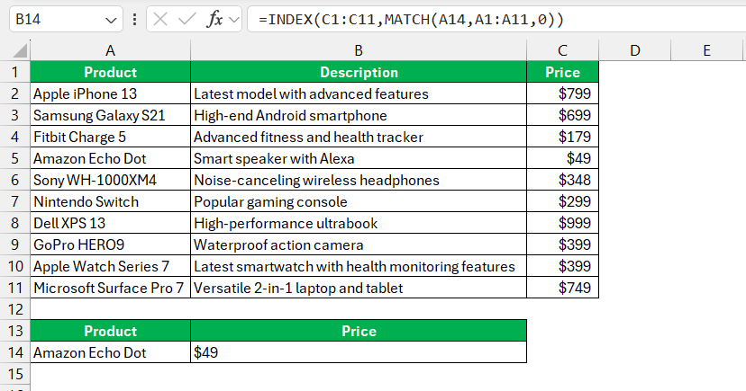
=INDEX(C1:C11, MATCH("Amazon Echo Dot", A1:A11, 0))

This formula searches for the term “Amazon Echo Dot” in the range A1:A11 and then returns the corresponding value from the same row in the range C1:C11.

The zero at the end of the MATCH function indicates you want an exact match—crucial for ensuring the precision of your lookup. With practice, you’ll find INDEX-MATCH to be vastly superior to VLOOKUP due to its flexibility and accuracy.

The importance of INDEX and MATCH comes into play when dealing with large data sets, where finding and matching data efficiently is crucial. By mastering these functions, you ensure that no matter how your spreadsheet evolves or how complex your data becomes, you can retrieve just the information needed with pinpoint accuracy.

 

Advanced Techniques to Extract Cell Values

Creating Dynamic Cell References with INDIRECT and ADDRESS

When it comes to managing spreadsheets with changing data points or structures, creating dynamic cell references with INDIRECT and ADDRESS is like having a superpower. The combination of these two functions fosters the creation of flexible formulas that adapt automatically to your data’s fluid nature.

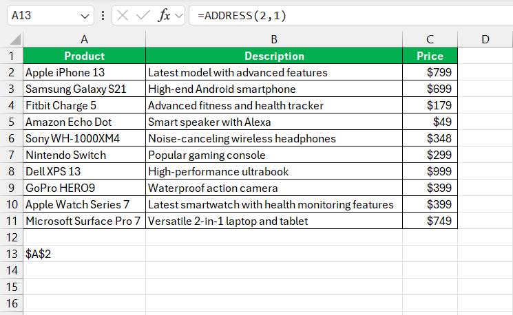
The ADDRESS function generates a cell address as text, using specified row and column numbers. It’s the first step in setting the stage for dynamism in your spreadsheet. Here’s its basic syntax: =ADDRESS(row_number, column_number)

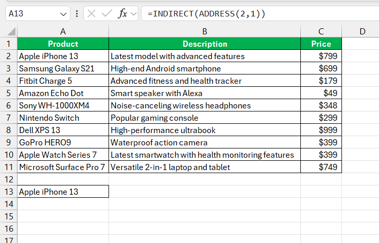
The INDIRECT function then takes the show by converting the text string obtained from ADDRESS into a cell reference that Excel recognizes and can interact with. This allows you to build formulas that reference various cells that might change position or be specified in some indirect way. For example: =INDIRECT(ADDRESS(2, 1))

Breaking it down, here’s why this combo is particularly handy:

• It enables flexibility in referencing cells that aren’t hard-coded into your formulas. Say goodbye to tedious manual updates of cell references in formulas when adding or removing rows and columns.
• INDIRECT and ADDRESS are perfect for creating named ranges that expand dynamically or for referencing cells in other worksheets dynamically.
• Keep in mind that INDIRECT is a volatile function. This means it recalculates whenever any change is made in the workbook, which can slow down large or complex workbooks. Balance its use against the benefit of dynamic referencing it provides.

Creating dynamic cell references becomes essential when dealing with models or reports that require constant updating and where manual editing could lead to errors or omissions. Embrace INDIRECT and ADDRESS, and you empower your spreadsheets to be more intelligent and responsive to your ever-changing data landscape.

 

Excel Formula Efficiency and Best Practices

Avoiding Common Pitfalls in Formula Creation

Creating formulas in Excel might seem simple, but even seasoned users can encounter common pitfalls that disrupt workflow or spoil data analysis. To ensure accuracy and efficiency, avoid these common mistakes:

• Using hard-coded values: This reduces flexibility. Instead, use cell references to allow automatic updates with changes to input values.
• Mismatched parentheses: Each open parenthesis needs a closing one. Missing one can cause errors and incorrect calculations.
• Confusing absolute and relative references: Mixing up absolute ($A$1) and relative (A1) references can cause issues when copying formulas. Use $ to lock cells and ensure consistency.
• Not updating range references: When adding new data, update the range within your formulas. Use dynamic named ranges or Excel Tables to automate this.
• Ignoring error checking: Excel’s built-in error checking can catch common mistakes. Watch for error flags and use tools like ‘Trace Precedents’ and ‘Trace Dependents’ to troubleshoot.

By paying close attention to these details, you can avoid frequent errors and ensure your analysis is reliable and accurate.

Tips for Maintaining Clean and Readable Spreadsheets

Maintaining clean and readable spreadsheets is not just about aesthetics; it’s pivotal for accuracy, ease of use, and facilitating collaboration. Here are crisp tips to keep your workbooks pristine and user-friendly:

• Organize with Consistency: Apply a consistent structure in terms of layout, fonts, and color schemes throughout your spreadsheet to make it intuitively navigable.
• Label Clearly: Make sure all columns, rows, and data sets have clear headings. Concise and descriptive labels help users understand data at a glance.
• Simplify Formulas: Break complex formulas into smaller parts across different cells, if feasible. This makes tracking the logic behind the calculations much easier.
• Utilize Cell Styles and Conditional Formatting: These features can highlight important information or alert you to outliers and errors, making the spreadsheet more interactive and accessible.
• Employ Data Validation: This feature ensures that data entries adhere to specified criteria, reducing the likelihood of errors due to incorrect data entry.

By adopting these strategies, your spreadsheets not only look better but also become more functional and less prone to error, making your Excel experience smoother and more productive.

 

FAQ: Expert Answers to Your Excel Questions

How do you show the value of a cell in Excel?

To show the value of a cell in Excel, simply click on the cell you are interested in. The value of the cell will appear in the cell itself and also in the formula bar at the top of the Excel window. If you want to display the value of a cell in another cell, use a formula like =A1, replacing A1 with the reference of the cell you’re interested in.

How to use the cell function in excel?

To use the CELL function in Excel, type =CELL(info_type, reference) into the cell where you want to display the information. Replace info_type with the kind of information you need (e.g., “address”, “format”, “contents”), and reference with the cell reference you’re inquiring about. For instance, =CELL("format", A1) will return the number format of cell A1.

How can I change a cell reference to a named range?

To change a cell reference to a named range in Excel, first select the range of cells you want to name. Then, go to the Name Box, located to the left of the formula bar, and type the name you wish to assign to that range. Press Enter to apply the name. Now you can use the named range instead of the cell reference in your formulas.

What are some common uses of the VALUE function in Excel?

The VALUE function in Excel is chiefly used for converting text strings that represent numbers into numeric values. Common uses include:

• Preparing Data for Calculations: Transforming imported data that’s formatted as text into numbers so they can be used in mathematical operations.
• Cleaning Data: Converting numbers stored as text, often due to formatting issues, to a numeric datatype to standardize datasets.
• Data Validation: Ensuring text entered as values can be appropriately used in formulas and calculations, avoiding the #VALUE! error.

What is #value in Excel cell?

The #VALUE! error in Excel signals a problem with the way your formula is typed or the cells you’re referencing in it. It typically appears when Excel expects a number but finds text or when a formula is applied to cells containing different data types that cannot be used together in calculations. Adjusting the formula’s syntax and ensuring consistent cell data types usually resolves the #VALUE! error.