Best Guide on How to Extract Text with Substring Functions in Excel

Unlock the potential of Microsoft Excel with a guide to its substring functions, which allow for sophisticated text manipulation. By understanding how to extract text from larger strings, users can enhance data management, streamline processes, and unlock deeper insights from their spreadsheets.

Key Takeaways:

• Substring functions, including LEFT, MID, and RIGHT, are essential for extracting specific text segments from larger strings, aiding in precise data analysis.
• Advanced functions like FIND, SEARCH, SUBSTITUTE, and REPLACE extend Excel’s text manipulation capabilities, allowing for more nuanced and complex operations.
• Data cleansing tools, such as TRIM and CLEAN, are critical for maintaining data integrity by removing extra spaces and non-printable characters.
• Text to Columns and Flash Fill automate the separation of combined data into individual columns and the filling of patterns, respectively, significantly reducing manual workload.
• TEXTBEFORE and TEXTAFTER functions offer high precision in extracting text segments based on specified delimiters, streamlining tasks that require detailed text extraction.

 

Unveiling the Excel Magic: Introduction to Substring Functions

What Is a Substring in Excel?

A substring in Excel might sound like a fancy term, but it’s really quite simple: it’s any portion of text pulled from a larger string of characters in a cell. Imagine each cell in your spreadsheet as a book—then a substring would be like a quote you’ve pulled from a page in that book. It could be a word, a sentence, or even a character—anything that’s part of the full text.

How to Extract Text Enhances Data Management

Extracting text in Excel is like finding treasure in the sandbox; it empowers you to sift through and retrieve only the most valuable data from a sea of information. By using substring functions correctly, you navigate through vast datasets with ease, promoting better organization, clearer analyses, and stronger reporting. Essentially, they help turn your raw data into refined, insightful gems.

The Essential Substring Trio: LEFT, RIGHT, MID

Using the LEFT Function for Text Extraction

Dive into the ease of text extraction with the LEFT function in Excel, which allows you to cut and harvest text from the leftmost part of a cell’s content. For instance, if you need to pluck out area codes or product categories that are always positioned at the start, the LEFT function is your go-to tool. Seamlessly copy the formula down a column, and voilà!—the desired characters appear neatly extracted for your review.

To extract using the LEFT function, enter =LEFT(Cell, Number_of_characters), like this: =LEFT(A1,4). Just replace ‘Cell’ with the cell containing your text, and ‘Number_of_characters’ with the exact number of characters you need.

 

Right into It: Harnessing the RIGHT Function

Flowing with the rhythm of data, the RIGHT function in Excel grabs the text from the string’s end, sort of like enjoying the best part of a song—the outro. It’s perfect for those moments when you need to extract serial numbers, dates, or any detail sitting snugly at the end of your cell’s content. You’ll marvel at how simple it is once you get the hang of using it!

To wield the RIGHT function effectively, your formula would look like =RIGHT(Cell, Number_of_characters). Just use =RIGHT(A1,4) and watch as Excel performs its magic, pulling the last four characters from the cell B5 into view. Remember, ‘Cell’ stands for the desired cell reference, and ‘Number_of_characters’ indicates how many characters from the end you want.

 

Crafting Mid-String Mastery with the MID Function

Between the Lines: Glimpse into MID’s Power

Envision being able to pluck out the juiciest part of a fruit—that’s what the MID function does with text in Excel. It’s a nifty tool that allows you to reach into the middle of a text string and extract the piece you need. Whether it be a part of a unique code, a specific detail within a comment, or a segment of an address, the MID function offers precision extraction from any position.

To craft your MID magic, the spell is =MID(text, start_position, number_of_chars). For example, =MID("pineapple",4,4) will fetch “eapp” from the center of “pineapple”. Here, ‘text’ is your full text string, ‘start_position’ is where you want to start extraction, and ‘number_of_chars’ is the length of the text you wish to extract.

 

Case Study Examples of MID in Action

Dive into the practical world of Excel with real-life examples that showcase the MID function’s versatility and strength. Imagine a company dealing with complex inventory SKUs, each string containing data such as product types, sizes, and colors in specific positions. Using the MID function, they successfully automate the extraction of each detail into separate columns, saving countless hours of manual work and minimizing the risk of human error.

Another scenario might involve a telecommunications provider analyzing call logs. With phone numbers and call durations embedded in lengthy text logs, the MID function enables the extraction of just the necessary digits for further analysis, aiding in customer service and operational improvements.

 

Beyond the Basics: Advanced Substring Tools

Find and Extract with FIND and SEARCH Functions

When LEGO pieces are mixed up, you need a keen eye to find the right one; this is akin to what the FIND and SEARCH functions do in your text-laden Excel spreadsheets. They both seek out specific characters or text within a cell, but with a twist—FIND is case-sensitive and does not play well with wildcards, while SEARCH is more relaxed, ignoring case differences and embracing wildcards like * and ?.

You could use FIND to pinpoint a first occurrence of a term with a formula like =FIND("Nemo","Finding Nemo"), which would return 9. Conversely, SEARCH would allow you to find the same word regardless of whether it is “nemo”, “Nemo”, or “NEMO”.

Remember, these functions find where the text is located, not the text itself. But when combined with other functions such as LEFT, RIGHT, or MID, you can extract substrings from right where they’re hiding.

 

Refining Text with the TRIM and CLEAN Functions

Imagine your text data as a garment needing a refresh. The TRIM function is your iron, smoothing out all the unnecessary spaces except the meaningful ones between words, giving your data a sharp, presentable look. With a simple =TRIM(A1), extra spaces are gone, and your text looks neat and uniform!

The CLEAN function, on the other hand, is like a stain remover, diligently removing invisible, non-printable characters that might have sneaked in during data import or copy-pasting. Cast the =CLEAN(A2) spell, and voilà, a spotless string of text remains.

Using TRIM and CLEAN together in Excel is a powerful combination for data cleansing, ensuring that what you analyze and report is as tidy and error-free as your perfectly organized spreadsheet cabinet.

 

Automate Wizardry: Flash Fill and Text to Column

Separating Data with Text to Columns Feature

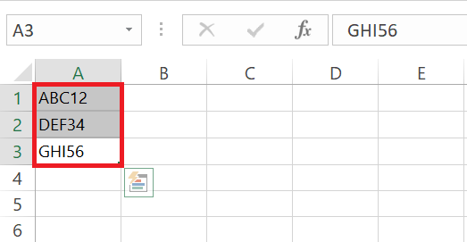
Tidying up data can feel like sorting a jumble of laundry—fortunately, Excel’s Text to Columns feature is the organizational wizard you need. It swiftly splits a column of combined information into neatly arranged, individual columns. With this feature, you can separate names, addresses, or any multi-part text with just a few clicks.

Here’s the magic formula:

STEP 1: Click on the column with the combined data you want to separate.

STEP 2: Navigate to Data > Data Tools > Text to Columns.

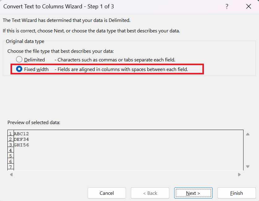
STEP 3: If your text is separated by commas, spaces, or another specific character, select ‘Delimited’. If it follows a fixed width, choose ‘Fixed Width’.

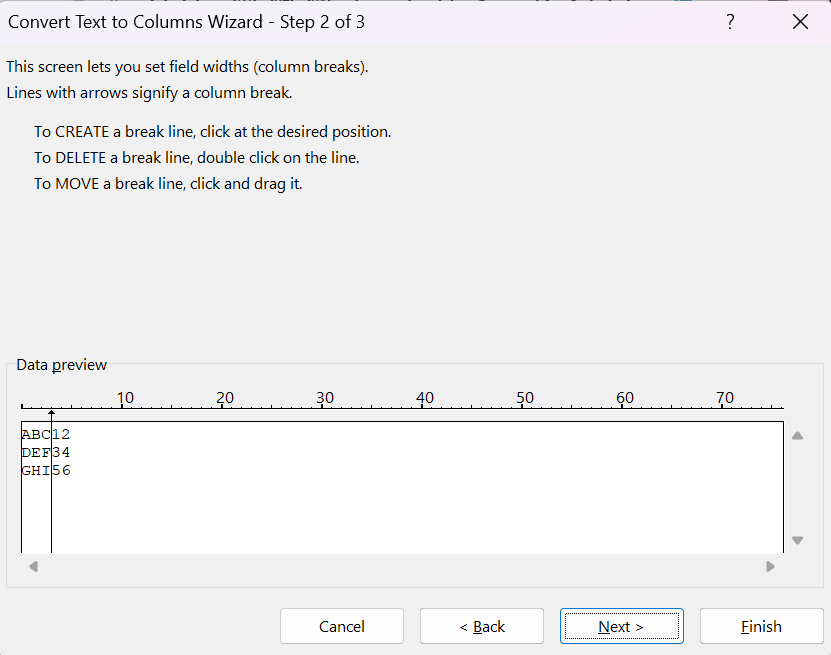
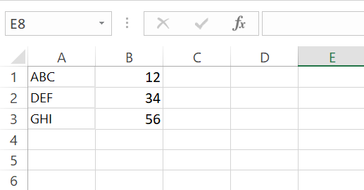
STEP 4: Excel previews your data separation. Tweak it if needed, and then click ‘Finish’ to see your data beautifully sorted into individual columns.

Check the result.

Whether you’re working with databases, mailing lists, or any list that could use some much-needed organization, Text to Columns transforms chaos into clarity—just like that!

 

Specialized String Operations for Expert Users

Digging Deeper with SUBSTITUTE and REPLACE Functions

Imagine being a text detective, looking for clues to decode a secret message. That’s what you do when you employ the SUBSTITUTE and REPLACE functions in Excel – both equip you to modify text strings, but each has its own specialty.

The SUBSTITUTE function is ideal when you need to swap out text based on its content. Think of changing dates formatted with dashes to slashes, or removing unwanted characters. It works like this: =SUBSTITUTE(text, old_text, new_text, [instance_num]). Specify the piece of text you want to replace, what you want to replace it with, and optionally, which occurrence to target.

 

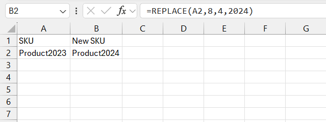
The REPLACE function, on the other hand, is like using precise coordinates to find a treasure. You tell Excel exactly where to start changing text and how many characters to replace. It goes like this: =REPLACE(old_text, start_num, num_chars, new_text). It’s perfect for when the location in the string, rather than the content, drives your edits.

Combining these functions can make your data manipulation in Excel not just quick, but also fun.

 

Employing TEXTBEFORE and TEXTAFTER for Precision

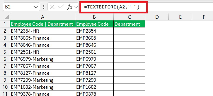
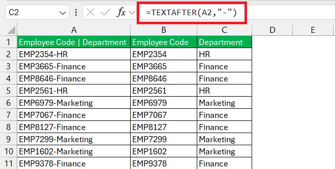
Excel’s TEXTBEFORE and TEXTAFTER functions are your high-precision tools, designed to extract text with the finesse of a skilled sculptor chiseling away to reveal the art within the stone. Whether you need to isolate a username from an email address or a product code from a full inventory number, these functions are your best allies for precise text extraction.

TEXTBEFORE zeroes in on the text before a specified delimiter. It follows the formula =TEXTBEFORE(text, delimiter, [instance_number], [if_not_found]). Perfect for situations where you need to extract everything before a certain character or word, like getting the domain from a list of URLs by specifying the delimiter as “/”.

TEXTAFTER, on the flip side, retrieves the text that comes after a particular character or string. Enter =TEXTAFTER(text, delimiter, [instance_number], [if_not_found]), and you can fetch the file extension from a filename by setting the delimiter to a dot.

These functions bridge the gap between cumbersome text manipulation and a sleek, automated process, turning hours of work into mere minutes.

 

FAQs Related to Excel Substring Functions

Q1: How do I retrieve text from a cell starting or ending with a specific character?

Use the RIGHT and LEFT functions in Excel to retrieve text starting or ending with a specific character. For the end part, use =RIGHT(cell, LEN(cell) - FIND("char", cell)), and for the start, =LEFT(cell, FIND("char", cell) - 1). Make sure to replace “cell” with your cell reference and “char” with your character.

Q2: Can I extract text from merged cells using substring functions?

Yes, you can extract text from merged cells using substring functions like LEFT, MID, and RIGHT by referencing the upper-left cell of the merged area. However, ensure your reference is consistent with merged cells‘ layout to avoid errors.

Q3: Are there any alternatives if standard substring functions don’t meet my requirements?

If standard substring functions fall short, you might explore add-ons like Ultimate Suite, using Flash Fill for pattern recognition, or dive into creating User-Defined Functions with VBA for custom solutions tailored to your needs.

Q4: How can I automate repetitive text extraction tasks in Excel?

To automate repetitive text extraction in Excel, use the Flash Fill feature for patterns, or record a Macro to apply a sequence of substring functions across multiple datasets speedily and consistently.

Q5 :How do I extract delimited text in Excel?

Use the Text to Columns feature in Excel to extract delimited text. Select your data, navigate to Data > Data Tools > Text to Columns, choose ‘Delimited’, select your specific delimiter, and click ‘Finish’.