Field List & Areas

Let us go over the different sections:

• Fields
• Rows
• Columns
• Values
• Report Filter

Exercise Workbook:

---

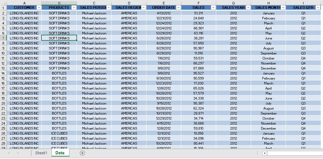
Here is our initial data table:

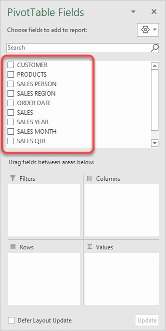
STEP 1: Now the first part is the Fields section, which represents the column headings of our data source:

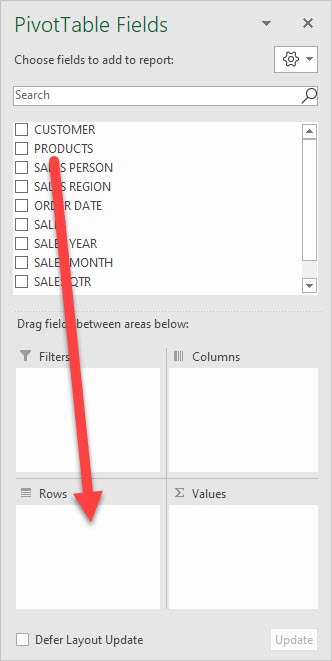
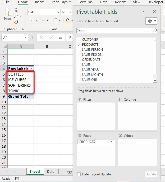
STEP 2: The Row labels show the unique fields on the left-hand side of our Pivot Table. Drag PRODUCTS to Rows to see how this looks like.

Now you can see our Products are listed on the Pivot Table.

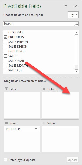
STEP 3: The Column labels show the trend of your data. For example, this could be periods, trends, time, month, years.

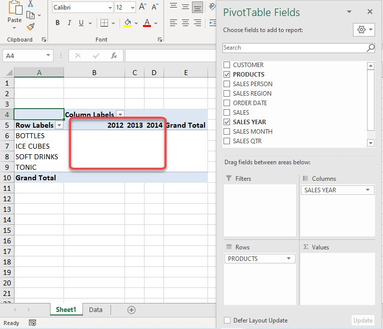
Let us drag the SALES YEAR to the Columns

Now you can see the years 2012 – 2014 as the columns.

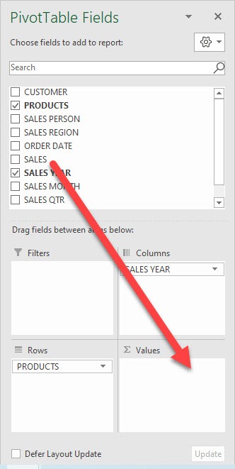
STEP 4: Values are fields that you want to calculate or quantify. Examples are sum (for sales), count (for number of units), average (for prices), and maximum/minimum (for values).

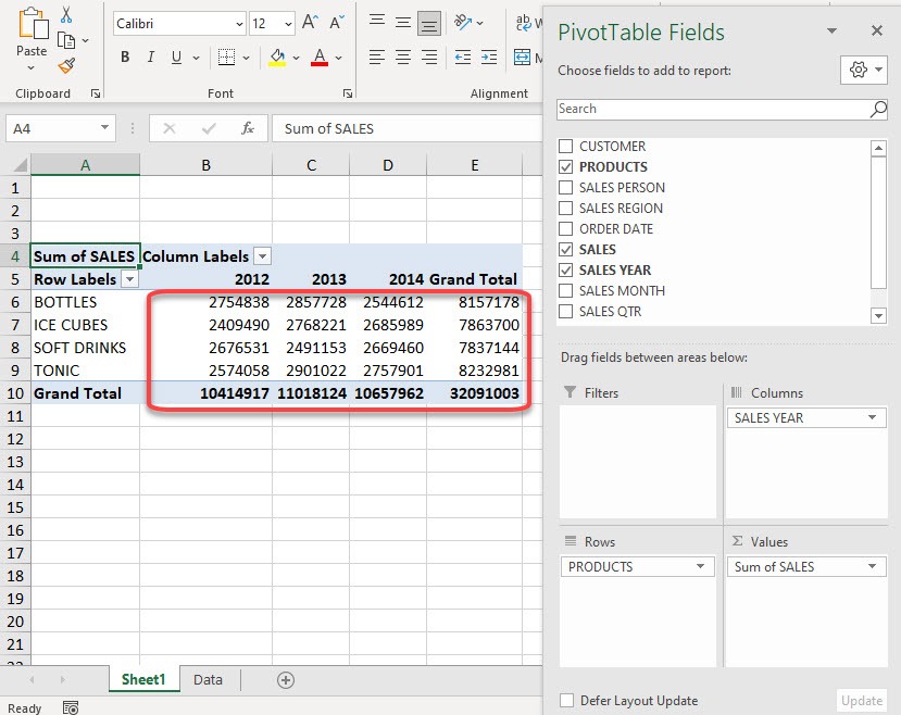
Let us drag SALES to Values

You will get the Sum of Sales values here for each Product-Year combination.

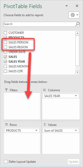
STEP 5: The last one is our Report Filters. These are optional fields that you want to drill down on. Examples are regions, periods, business units, or staff.

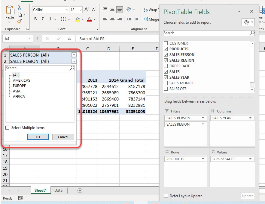
Drag both SALES REGION and SALES PERSON to the Filters area

Click on any filter and you will be able to filter your Pivot Table data according to your selection.

 

Make sure to download our FREE PDF on the 333 Excel keyboard Shortcuts here: