Field Name Formatting in Excel Pivot Tables

I will show you how to set up field name formatting in Excel Pivot Tables!

Exercise Workbook:

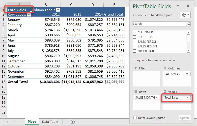
Here is our Pivot Table. We want to change the Sum of SALES to Total Sales for better readability.

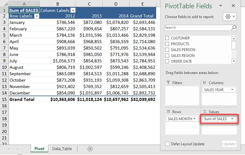
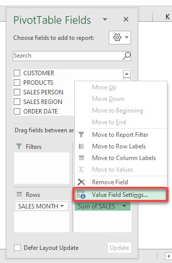
STEP 1: Click on the arrow beside Sum of SALES and select Value Field Settings

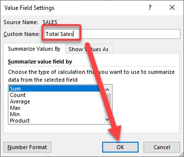
STEP 2: Type Total Sales for the Custom Name and click OK

Now you have Total Sales as your Field Name!

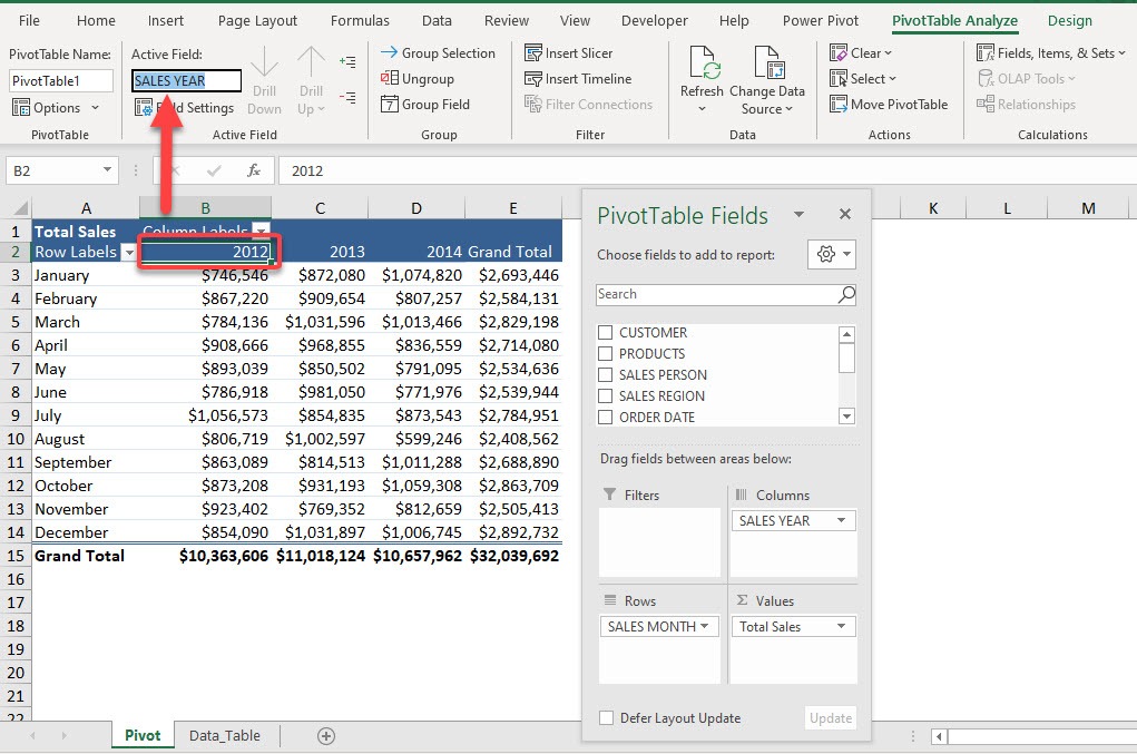
STEP 3: There is another way to do this. Now we want to change SALES YEAR to Financial Year

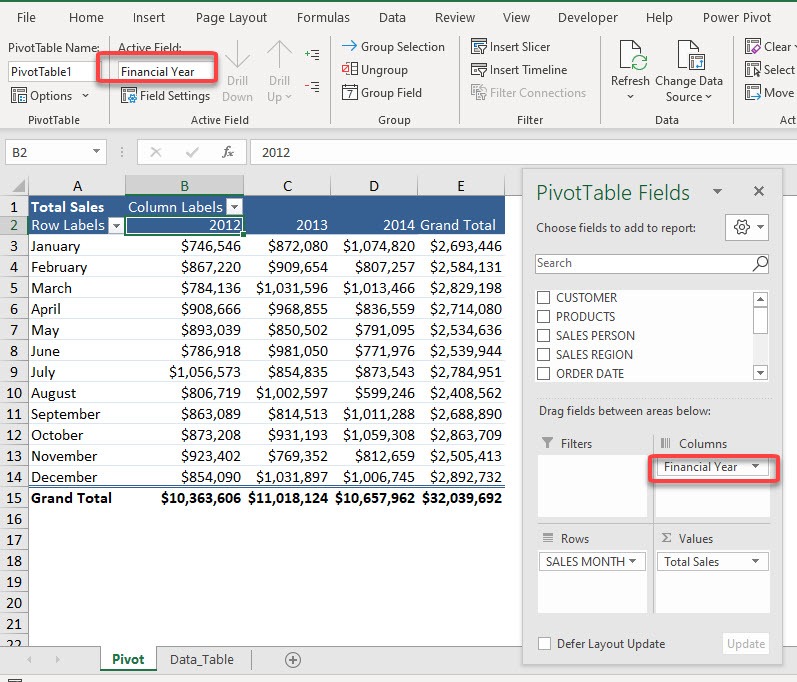
Select any SALES YEAR label in your Pivot Table. Go to PivotTable Analyze > Active Field > Active Field

Type in Financial Year as the new name:

And you can see your new field name take effect!

Make sure to download our FREE PDF on the 333 Excel keyboard Shortcuts here:

Bryan

Bryan Hong is an IT Software Developer for more than 10 years and has the following certifications: Microsoft Certified Professional Developer (MCPD): Web Developer, Microsoft Certified Technology Specialist (MCTS): Windows Applications, Microsoft Certified Systems Engineer (MCSE) and Microsoft Certified Systems Administrator (MCSA).

He is also an Amazon #1 bestselling author of 4 Microsoft Excel books and a teacher of Microsoft Excel & Office at the MyExecelOnline Academy Online Course.