Filter by Values – Between

 

Exercise Workbook:

---

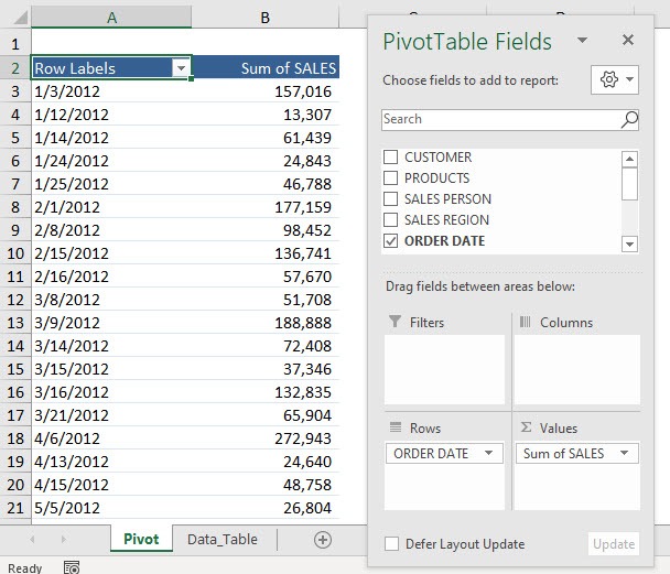
This is our current Pivot Table setup. We will be filtering the Sum of Sales amounts.

 

Example 1: Filter by Values – Between

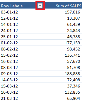
STEP 1: Click on the Row Label filter button in the Pivot Table.

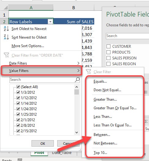
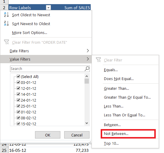
STEP 2: Select Value Filters.

You will see that we have a lot of filtering options. Let us try out – Between

STEP 3: Type in between 100000 and 200000. You can see that the Value Filter will be applied to the Sum of SALES.

Click OK

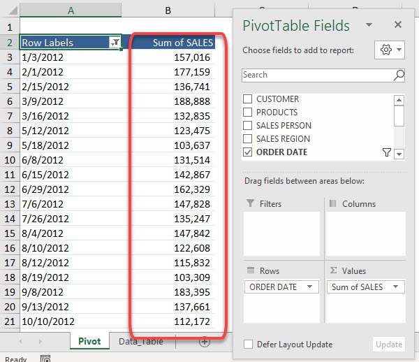
Now we have the filtering applied in a flash! The Sum of SALES values now displays the ones between 100,000 and 200,000.

 

Example 2: Filter by Values – Not Between

STEP 1: Click on the Row Label filter button in the Pivot Table.

STEP 2: Select Value Filters.

You will see that we have a lot of filtering options. Let us try out – Not Between

STEP 3: Type in between 2000 and 600000. You can see that the Value Filter will be applied to the Sum of SALES.

Click OK

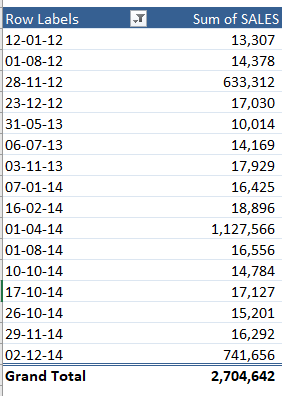
Now we have the filtering applied in a flash! The Sum of SALES values now displays the dates where the sum of sales is not between 20,000 and 600,000.

 

Following the steps mentioned above, you can easily filter the Pivot Table by values to get data between or not between a specific range. You can also use Pivot Table to filter Top/Bottom items by value or percentage, etc.

Click here to learn all about Pivot Tables.

 

Make sure to download our FREE PDF on the 333 Excel keyboard Shortcuts here: