Can you filter your table data using an Excel FILTER Formula? Yes, you can! It is definitely possible now with Excel FILTER Formula. It is a new formula introduced in Office 365 released in 2018!
Key Takeaways:
- The Excel FILTER function is a versatile tool that can be used for simple data filtering as well as for applying multiple criteria with OR & AND logic. It efficiently sorts and retrieves specific data sets from a larger pool, enhancing productivity significantly when paired with other Excel functions like VLOOKUP, SUMIF, and IF.
- The FILTER function is exceptionally beneficial for data analysis due to its ability to be combined with aggregation functions such as SUM, AVERAGE, COUNT, MAX, or MIN. This feature allows users to not only extract relevant data points but also to perform summary calculations for a specific group or subset of data.
- When using the FILTER function in Microsoft Excel, it is important to use a placeholder, such as zero, for the if_empty argument. This ensures that in cases where no data meets the established criteria, the function returns a ‘0’ instead of resulting in a #VALUE error. Careful use of the if_empty argument aids in obtaining cleaner results and avoiding unnecessary errors in your data analysis tasks.
Table of Contents
Excel Filter Formula
The FILTER formula in Excel is available in Office 365 only.
It is an in-built formula in Excel used to filter an array or range based on the criteria you specify and extract matching records.
It is part of Dynamic Array functions and the result provided by this formula is an array that spills on the worksheet automatically.
What does it do?
Filters a table array based on the filtering condition given
Formula breakdown:
=FILTER(array, include, [if_empty])
What it means:
- array – data to be filtered.
- include – logical test supplied as criteria. It should have the same height or width as the array.
- if_empty – value to display if the filter results in no records. It is an optimal argument.
Generally, Excel user filters data using the Autofilter button present under the Data Tab. But the drawback of using the filter buttons is that it does not update results automatically when you make changes in the data.
Whereas, the Excel FILTER function in Excel is dynamic i.e. when the values in the data sources change the result from this formula will update automatically.
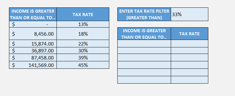
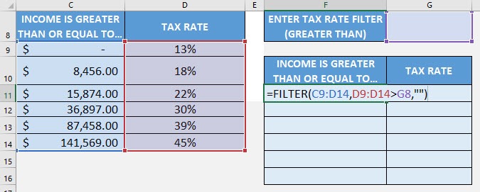
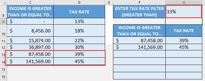
In the example below, we have a tax table that we want to dynamically filter with a given rate. So, we want to extract the income levels for which the tax rate is greater than 33%
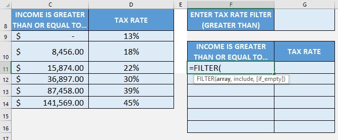
STEP 1: We need to enter the FILTER function in a blank cell:
=FILTER(
STEP 2: The Excel FILTER formula arguments:
array
What is the data to be filtered?
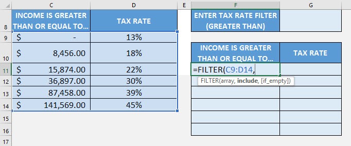
Select the cells containing the tax data, do not include the headers:
=FILTER(C9:D14,
include
What is your filtering condition?
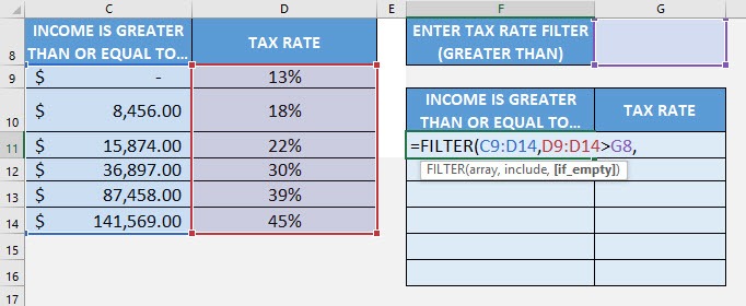
We want to filter the tax rate that is greater than the specified rate. Type in the condition as the tax rate column > the specific tax rate.
=FILTER(C9:D14, D9:D14>G8
[if_empty]
What is the value to display in case nothing gets matched?
Just place an empty string to be displayed if nothing gets matched.
=FILTER(C9:D14, D9:D14>G8, “”)
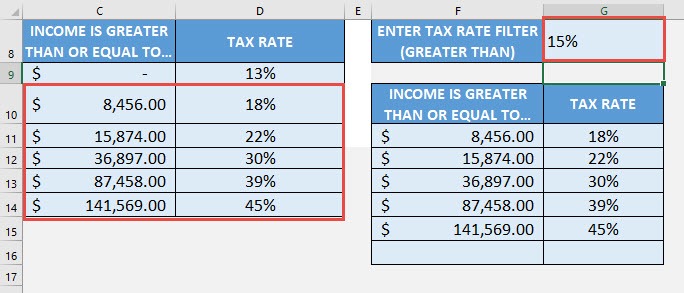
Try it out now with different values and see it get filtered magically!
This formula can handle multiple criteria as well. Let’s check it out!
Filtering with Multiple Criteria
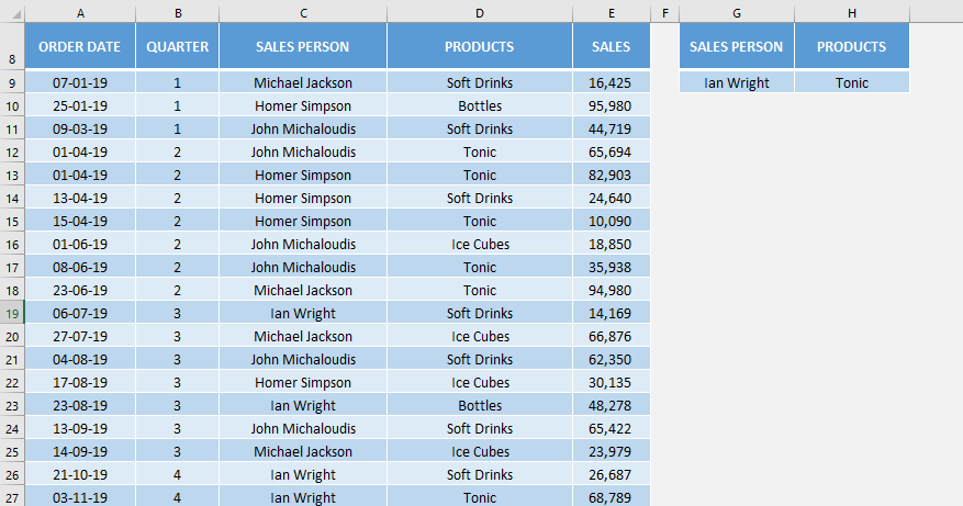
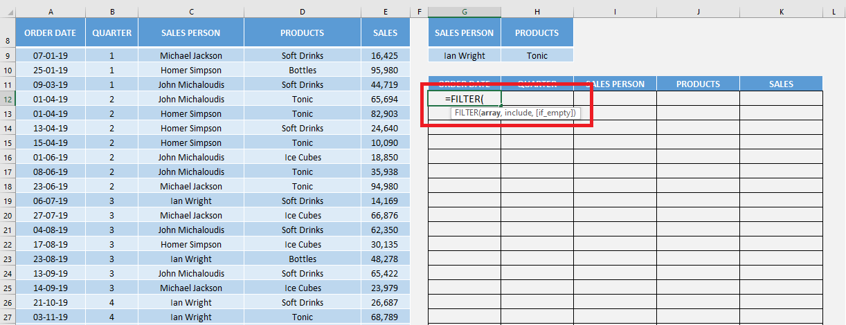
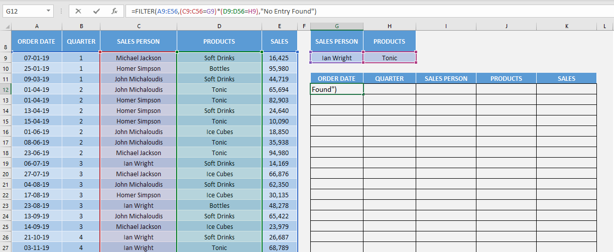
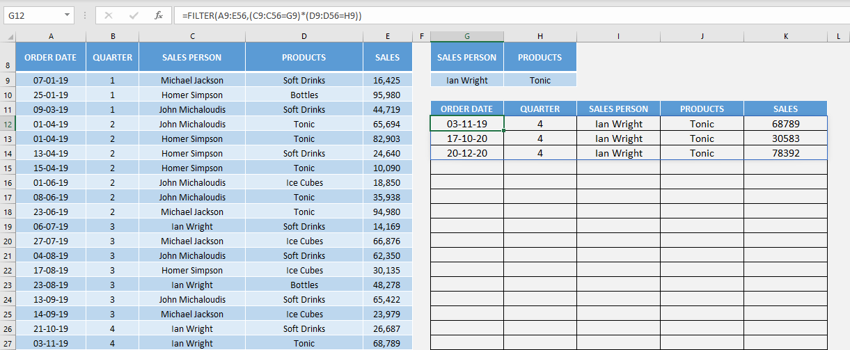
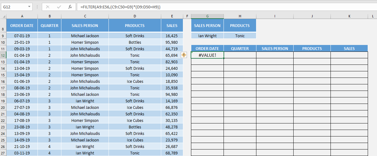
In this example, we have sales data and we want to filter data when the salesperson is Ian Wright and Product is Tonic.
Let’s use the FILTER formula wth multiple criteria and get this done!
STEP 1: Enter the FILTER function in cell G12.
=FILTER(
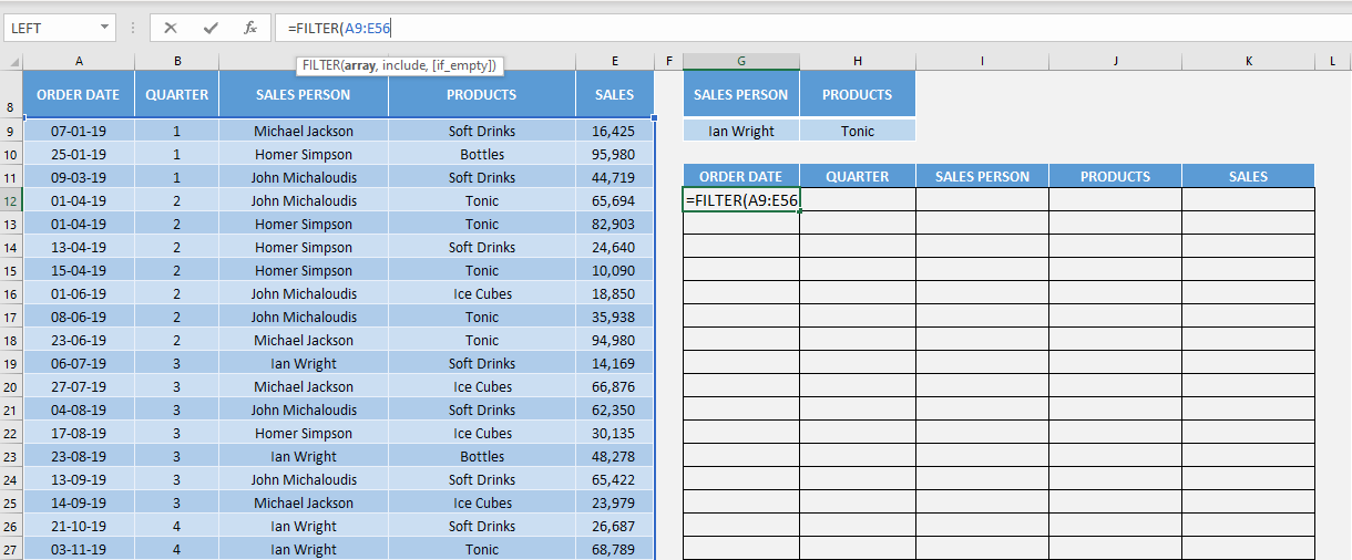
STEP 2: Select the array that needs to be filtered i.e. A9: E56
=FILTER(A9:E56
Now, you add multiple criteria you need to make sure that the two logical tests are separated by a multiplication operator.
=FILTER(array, (range1=criteria1) * (range2=criteria2))
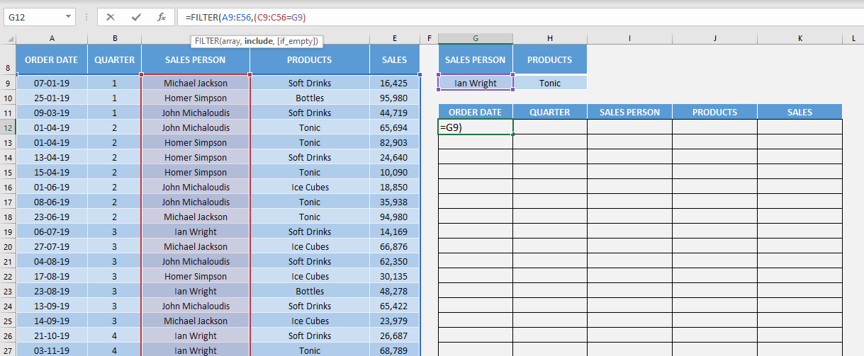
STEP 3: Add the first range (salesperson) and its criteria (Ian Wright) i.e. C9: C56 and G9 respectively.
=FILTER(A9:E56, (C9:C56=G9)
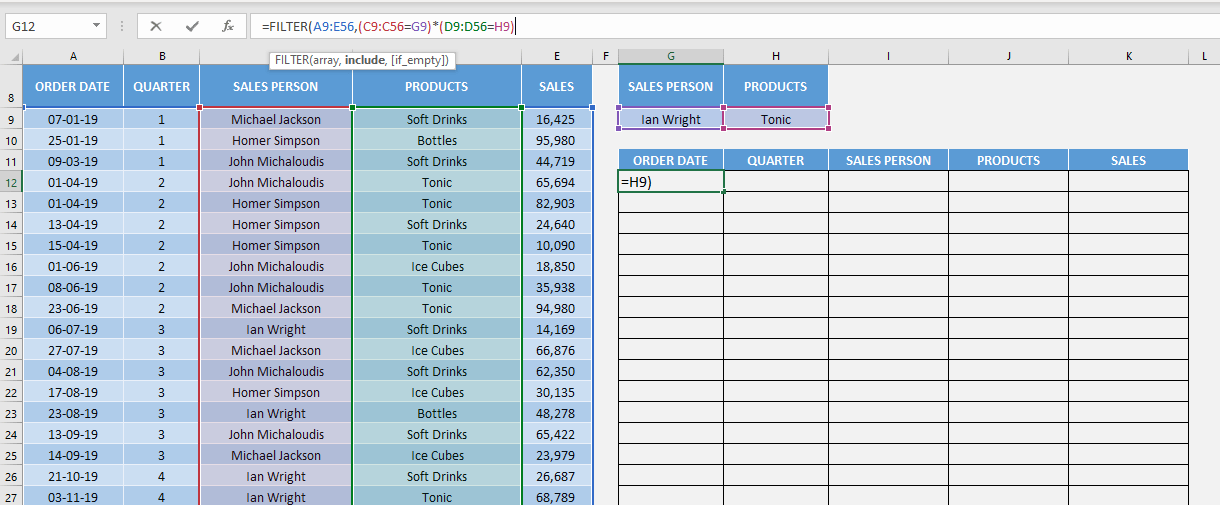
STEP 4: Insert a Multiplication Operator and then add the second range (product) and its criteria (Tonic) i.e. D9: D56 and H9 respectively.
=FILTER(A9:E56, (C9:C56=G9) *(D9:D56=H9)
STEP 5: Add the text to display if the filtering results in no record i.e. No Entry Found.
=FILTER(A9:E56, (C9:C56=G9) *(D9:D56=H9),”No Entry Found”)
This is how you can use the Excel FILTER formula with single or multiple criteria.
Byt, there may be times when you might encounter an error when using filter function Excel. Let’s look at some of those errors and how to correct them!
Filter formula not working
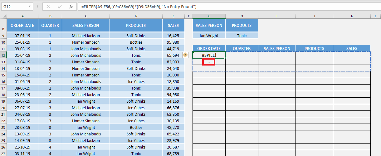
#SPILL Error
This error occurs if one or more cells where the result will be displayed in not blank.
In this example, as you can see there is already text (-) in cell G13. The FILTER formula is showing error.
To fix it, simply delete any contents present in those cells and the desired result will appear.
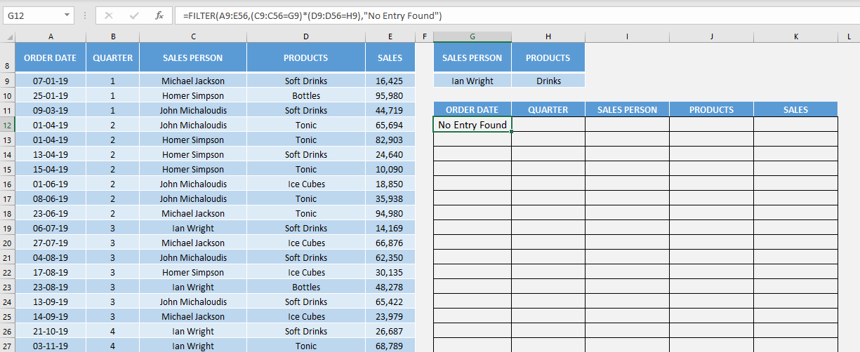
#CALC! Error
This error occurs when if_empty is omitted and there is no entry matching the criteria provided.
In this example, as you can see there is no text present of if_empty argument and there are no records for salesperson Ian Wright and product Drinks, there is an #CALC! error.
To fix it, simply add a text in the formula’s if_empty argument.
#VALUE Error
One of the reasons why no may encounter this error is that neither the height or width of the include argument matches that of the array argument.
In this example, the height of the array is from row 9 to row 56 but height for include is for row 9 to row 50. So, Excel displays an #VALUE! error!
To fix it, simply make sure that the height or width of include is the same as the array.
Integrating Excel’s Dynamic Array Functions
Combining FILTER with UNIQUE and SORT
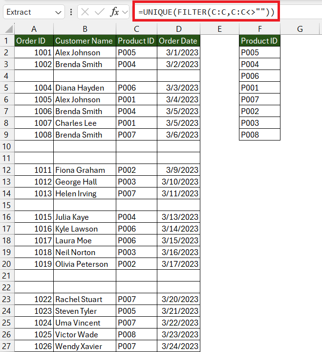
The synergy between Excel’s FILTER, UNIQUE, and SORT functions unlocks dynamic array capabilities that can revolutionize how you manage data. Imagine you have a list of sales data, including duplicates. With the FILTER function, you can swiftly extract only the relevant records matching specific criteria. Now, blend in the UNIQUE function, and voilà, your list is pruned to show only unique occurrences, free from repetitive entries.
But why stop there? Casting the SORT function into the mix organizes your filtered, unique list into an orderly fashion. The result? A data set that’s not only tailored to your needs but also neatly arranged.
For example, let’s visualize a data set containing information about different fruits and their corresponding sales in various regions. After applying the FILTER function to isolate fruits with sales above a particular threshold, the list might still show multiple entries per fruit. The UNIQUE function then ensures that each fruit appears only once. Lastly, using SORT can alphabetically order the fruits or sort them by sales volume, providing clear insights at a glance.
Here’s a snapshot of these functions in powerful collaboration:
- FILTER ensures you see only rows that meet your criteria.
- UNIQUE then removes any duplicates from the filtered results.
- SORT orders the resulting array, providing streamlined data retrieval.
By mastering this trifecta, you’ll elevate your data analysis game, distilling large, complex datasets into actionable insights with just a few simple formulas.
Creative Uses of FILTER with Functions like MID, FIND, and LAMBDAs
Excel’s FILTER function is like a data magician’s assistant, but when you pull other functions from your hat, such as MID, FIND, and LAMBDA, it’s pure prestidigitation! These functions transform FILTER into an even more potent analytical tool, allowing you to sift through data with precision and creativity.
Take MID and FIND, for instance. They specialize in string manipulation and searching, respectively. When combined with FILTER, they empower you to perform partial text matches, making it possible to filter data based on specific text fragments. This is particularly handy when dealing with product codes, names, or any data that contains a consistent structure.
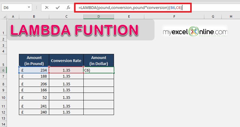
For the more advanced Excel wizards, there’s LAMBDA, a function that creates custom, reusable functions without the need for VBA. You can craft your own filters that address complex, repetitive tasks and summon them at will across your workbook.
Envision a scenario where you’re dealing with a vast inventory list and you’re looking for items where a certain code appears in the middle of their reference IDs. By employing FILTER with MID and FIND, you can isolate these items quickly. Or perhaps you’ve created a LAMBDA function to assess sales data, and you need to apply specific, repeated analytical filters unique to your dataset—this is where LAMBDA makes the magic happen.
These creative combinations foster innovation in data manipulation, pushing the boundaries of what’s possible in Excel, transforming your data analysis into an art form.
FAQ: Unlocking the Secrets of Excel Filter Formulas
What are the most common mistakes when using the Excel FILTER function?
The most common pitfalls encountered when casting spells with the Excel FILTER function include mismatched ranges, where the columns you’re trying to filter don’t align in size — leading to a spellcasting misfire. Also, using dynamic ranges or tables can help prevent such mismatches as they adapt to data changes automatically. Another frequent error stems from neglecting empty cells, which can skew results or even prevent the function from executing properly.
Remember, a well-structured incantation requires uniform data entry and crystal-clear labeling for each column to avoid confusion and maximize the FILTER function’s potential. Keep these tips in mind, and you’ll have your data dancing to your tune without a hitch.
Can I use the Excel FILTER function to display top or bottom records?
Absolutely! The FILTER function can sort your data to display top or bottom records by ingeniously combining it with other Excel functions like SORT and SORTBY. With this formula fusion, you’re able to summon an ordered list that can easily display either the highest or lowest values in your dataset. This is particularly useful when you’re seeking to identify peak performers or areas that require improvement.
To display the top records, such as the highest sales figures, combine FILTER with SORT in descending order. Conversely, show bottom records like the least sales by sorting in ascending order.
In essence, by weaving together the FILTER with SORT or SORTBY, your data will reveal the cream of the crop or those at the bottom, all depending on your needs.
How can I avoid #SPILL! errors when working with Excel filters?
To banish the dreaded #SPILL! error while conjuring formulas with Excel’s FILTER function, keep the surrounding cells clear of any data or text. Always ensure there’s ample space for the function to spill its results; think of it like giving your magic room to breathe.
If new entries require a larger spill area, structure your data as an Excel table or dynamic named range to adapt to changes gracefully. These proactive measures keep the #SPILL! curse at bay, allowing your data to flow seamlessly across your spreadsheet.

Bryan
Bryan Hong is an IT Software Developer for more than 10 years and has the following certifications: Microsoft Certified Professional Developer (MCPD): Web Developer, Microsoft Certified Technology Specialist (MCTS): Windows Applications, Microsoft Certified Systems Engineer (MCSE) and Microsoft Certified Systems Administrator (MCSA).
He is also an Amazon #1 bestselling author of 4 Microsoft Excel books and a teacher of Microsoft Excel & Office at the MyExecelOnline Academy Online Course.
